• My summer goal was to blog more. So here I go. Two posts in two days. No way can I keep that pace up.

    So I recently had the chance to teach a short course on web scraping and text analysis.  One of my examples scraped data from presidential inaugural speeches.  With this corpus (a new word that I learned), we can look at things like the most often used words


    findFreqTerms(presTDM,300) 
    [1] "can" "government" "great" "may" "must" "people" 
    [7] "shall" "states" "upon" "will"


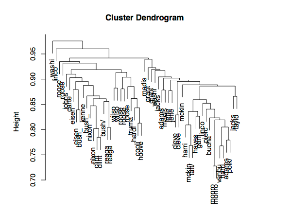
    I then used to demonstrate some clustering methods.  For instance, using hierarchical clustering will produce a dendrogram like the following:
    Screen Shot 2014-06-03 at 6.57.10 PM

    The data to make this plot consists of a large sparse matrix with each row representing a speech and each column corresponding to a word with a count of the number of times the j-th word was used in the i-th speech.  In this way you can measure the distance between each speech and do clustering.

    As it turned out I had some political science students in the class and they pointed out to me that it looks like there are two big groups consisting of recent presidents and less recent presidents.  So the question came up as to what was the difference?

    So on the fly I write some code to test for differences in word use between the older and newer presidents.  What we ended up doing was a two sample t-test for each word split by old or new president. These groups were created by putting all presidents prior to and including Taft into group 1 and all presidents after Taft into group 2.

    We then recorded the p-value for each of these tests. If we used a level alpha=0.05 for family wise error rate, a Bonferroni corrected threshold would be 5.604753e-06. Three words reached this conservative cut-off: duties, world, and public. The top 100 words (I removed january and march since those are dates of the speeches and don’t really count) based on p-values appear below.


                            word         pval
    duties                 duties 4.629343e-07
    world                   world 1.095059e-06
    public                 public 4.391972e-06
    subject               subject 9.420443e-06
    today                   today 1.256848e-05
    america               america 1.568912e-05
    know                     know 1.787979e-05
    live                     live 2.668409e-05
    life                     life 2.895837e-05
    regard                 regard 3.306319e-05
    lives                   lives 4.643304e-05
    interests           interests 4.711251e-05
    foreign               foreign 4.855870e-05
    objects               objects 4.948200e-05
    functions           functions 5.686164e-05
    help                     help 6.199250e-05
    work                     work 6.522966e-05
    present               present 6.926184e-05
    attention           attention 7.776694e-05
    peculiar             peculiar 9.771913e-05
    civil                   civil 1.016519e-04
    states                 states 1.018945e-04
    views                   views 1.055752e-04
    condition           condition 1.336558e-04
    unity                   unity 1.368429e-04
    general               general 1.475924e-04
    virtue                 virtue 1.920787e-04
    come                     come 1.976854e-04
    enjoyed               enjoyed 2.605138e-04
    happily               happily 2.605138e-04
    settled               settled 2.628839e-04
    discharge           discharge 2.770679e-04
    opportunity       opportunity 2.981866e-04
    god                       god 3.266714e-04
    old                       old 3.336640e-04
    execute               execute 3.378849e-04
    new                       new 3.598835e-04
    vision                 vision 3.746672e-04
    opinion               opinion 3.992428e-04
    wise                     wise 4.278589e-04
    centuries           centuries 5.185043e-04
    enable                 enable 5.608008e-04
    americans           americans 6.192669e-04
    official             official 6.339651e-04
    original             original 6.970246e-04
    station               station 7.021808e-04
    strict                 strict 7.021808e-04
    constitution     constitution 7.404890e-04
    therefore           therefore 7.463164e-04
    state                   state 7.476751e-04
    way                       way 8.538455e-04
    gods                     gods 8.743461e-04
    nation                 nation 8.817792e-04
    object                 object 8.921927e-04
    women                   women 8.977030e-04
    none                     none 9.039120e-04
    portion               portion 9.805345e-04
    patriotic           patriotic 9.942662e-04
    freedom               freedom 1.020410e-03
    liberal               liberal 1.155951e-03
    importance         importance 1.160502e-03
    together             together 1.174523e-03
    judgment             judgment 1.285434e-03
    vice                     vice 1.285803e-03
    faithful             faithful 1.343211e-03
    existence           existence 1.419454e-03
    gratitude           gratitude 1.457342e-03
    cultivate           cultivate 1.464136e-03
    attained             attained 1.464136e-03
    entertained       entertained 1.464136e-03
    scarcely             scarcely 1.580568e-03
    economic             economic 1.597010e-03
    several               several 1.617976e-03
    may                       may 1.725435e-03
    build                   build 1.781003e-03
    poverty               poverty 1.781003e-03
    intercourse       intercourse 1.782419e-03
    circumstances   circumstances 1.812426e-03
    dignity               dignity 1.820683e-03
    born                     born 2.016370e-03
    patriotism         patriotism 2.039916e-03
    need                     need 2.077322e-03
    resolve               resolve 2.203595e-03
    administration administration 2.250915e-03
    blessings           blessings 2.253577e-03
    formed                 formed 2.277049e-03
    officers             officers 2.315975e-03
    administered     administered 2.365768e-03
    assembled           assembled 2.365768e-03
    heretofore         heretofore 2.365768e-03
    historic             historic 2.511711e-03
    exists                 exists 2.662722e-03
    felt                     felt 2.763852e-03
    domestic             domestic 2.773740e-03
    debt                     debt 2.835649e-03
    disposition       disposition 2.850068e-03
    policy                 policy 2.851784e-03
    

    Of course this test was only looking at differences and it doesn’t answer which direction the difference is in. Let’s look at a few of the top words (Note: group2 is more recent president):

     t.test((m[,colnames(m)=="duties"])~group)
    
    	Welch Two Sample t-test
    
    data:  (m[, colnames(m) == "duties"]) by group
    t = 6.1796, df = 34.719, p-value = 4.629e-07
    alternative hypothesis: true difference in means is not equal to 0
    95 percent confidence interval:
     1.651399 3.267956
    sample estimates:
    mean in group 1 mean in group 2 
           2.709677        0.250000 
    
    
    t.test((m[,colnames(m)=="world"])~group)
    
    	Welch Two Sample t-test
    
    data:  (m[, colnames(m) == "world"]) by group
    t = -6.4016, df = 24.814, p-value = 1.095e-06
    alternative hypothesis: true difference in means is not equal to 0
    95 percent confidence interval:
     -10.86082  -5.57198
    sample estimates:
    mean in group 1 mean in group 2 
           1.741935        9.958333 
    
    t.test((m[,colnames(m)=="public"])~group)
    
    	Welch Two Sample t-test
    
    data:  (m[, colnames(m) == "public"]) by group
    t = 5.1556, df = 49.692, p-value = 4.392e-06
    alternative hypothesis: true difference in means is not equal to 0
    95 percent confidence interval:
     2.921318 6.651263
    sample estimates:
    mean in group 1 mean in group 2 
            6.16129         1.37500
    

    The word “duties” was used on average about 2.7 times in older inaugural addresses and only .25 times in the newer speeches.

    The word “world” was used on average about 1.74 times per inaugural address among the old speeches, whereas in the newer speeches it was used on average about 9.96 times per address. Below is a break down of who was using the word “world”.

    m[,colnames(m)=="world"]
    washi washi adams jeffe jeffe madis madis monro monro adams jacks jacks vanbu 
        1     0     3     2     2     2     1     0     2     1     0     2     2 
    harri polk/ taylo pierc bucha linco linco grant grant hayes garfi cleve harri 
        2     5     0     3     3     1     1     1     2     2     2     1     0 
    cleve mckin mckin roose taft/ wilso wilso hardi cooli hoove roose roose roose 
        0     6     2     3     2     2     6    23    13    14     6     1     3 
    roose truma eisen eisen kenne johns nixon nixon carte reaga reaga bush/ clint 
        2    22    14    14     8     7    12    16     5     8    14    10    18 
    clint bush_ bush_ 
       10     3     8 
    

    Finally, the word “public” was used about 6.16 times in the old addresses and only 1.375 times in the new address.

    Further down the list, the word “god” shows up (Note: all words have been forced to lowercase).

    t.test((m[,colnames(m)=="god"])~group)
    
    	Welch Two Sample t-test
    
    data:  (m[, colnames(m) == "god"]) by group
    t = -3.9492, df = 38.157, p-value = 0.0003267
    alternative hypothesis: true difference in means is not equal to 0
    95 percent confidence interval:
     -2.4558401 -0.7914717
    sample estimates:
    mean in group 1 mean in group 2 
          0.7096774       2.3333333 
    

    And we we look at which group is using the word more often, we see that in the older addresses the word “god” was used on average about .71 times per address, whereas in the newer speeches it is used 2.33 times per address. If we break this down by speech it’s even more interesting.

    > m[,colnames(m)=="god"]
    washi washi adams jeffe jeffe madis madis monro monro adams jacks jacks vanbu 
        0     0     0     0     0     0     0     0     1     0     0     0     0 
    harri polk/ taylo pierc bucha linco linco grant grant hayes garfi cleve harri 
        0     0     0     1     1     0     5     1     0     0     3     1     2 
    cleve mckin mckin roose taft/ wilso wilso hardi cooli hoove roose roose roose 
        2     2     2     0     1     1     1     4     1     2     2     0     1 
    roose truma eisen eisen kenne johns nixon nixon carte reaga reaga bush/ clint 
        2     2     4     1     2     3     5     2     1     4     8     2     1 
    clint bush_ bush_ 
        1     3     3 
    

    The word “god” wasn’t mentioned in any of the first 8 presidential inaugural addresses and only 3 times in the first 18. In fact it wasn’t until Lincoln where the word god was used more than once. Every president since Garfield has mentioned the word “god” in their inaugural address at least once with the exception of Teddy Roosevelt and FDR (second address). And Reagan used the word “god” 8 times in his second inaugural address.

    I also though the words “drugs” and “work” were interesting so I added those here:

    m[,colnames(m)=="drugs"]
    washi washi adams jeffe jeffe madis madis monro monro adams jacks jacks vanbu 
        0     0     0     0     0     0     0     0     0     0     0     0     0 
    harri polk/ taylo pierc bucha linco linco grant grant hayes garfi cleve harri 
        0     0     0     0     0     0     0     0     0     0     0     0     0 
    cleve mckin mckin roose taft/ wilso wilso hardi cooli hoove roose roose roose 
        0     0     0     0     0     0     0     0     0     0     0     0     0 
    roose truma eisen eisen kenne johns nixon nixon carte reaga reaga bush/ clint 
        0     0     0     0     0     0     0     0     0     0     0     1     0 
    clint bush_ bush_ 
        2     0     0 
    
    m[,colnames(m)=="work"]
    washi washi adams jeffe jeffe madis madis monro monro adams jacks jacks vanbu 
        0     0     0     1     0     0     1     3     0     1     0     0     1 
    harri polk/ taylo pierc bucha linco linco grant grant hayes garfi cleve harri 
        1     0     0     0     1     0     1     0     0     1     1     1     1 
    cleve mckin mckin roose taft/ wilso wilso hardi cooli hoove roose roose roose 
        2     2     1     1     7     2     0     2     2     1     3     3     0 
    roose truma eisen eisen kenne johns nixon nixon carte reaga reaga bush/ clint 
        2     4     6     2     1     3     0     4     2     7     5     7     6 
    clint bush_ bush_ 
        8     4     6 
    

    And finally, here’s a word cloud of all the words used in the inaugural addresses because everyone loves word clouds.
    Screen Shot 2014-06-03 at 6.56.21 PM

    Cheers.

  • Per the request of @M_T_Patterson and @statsByLopez

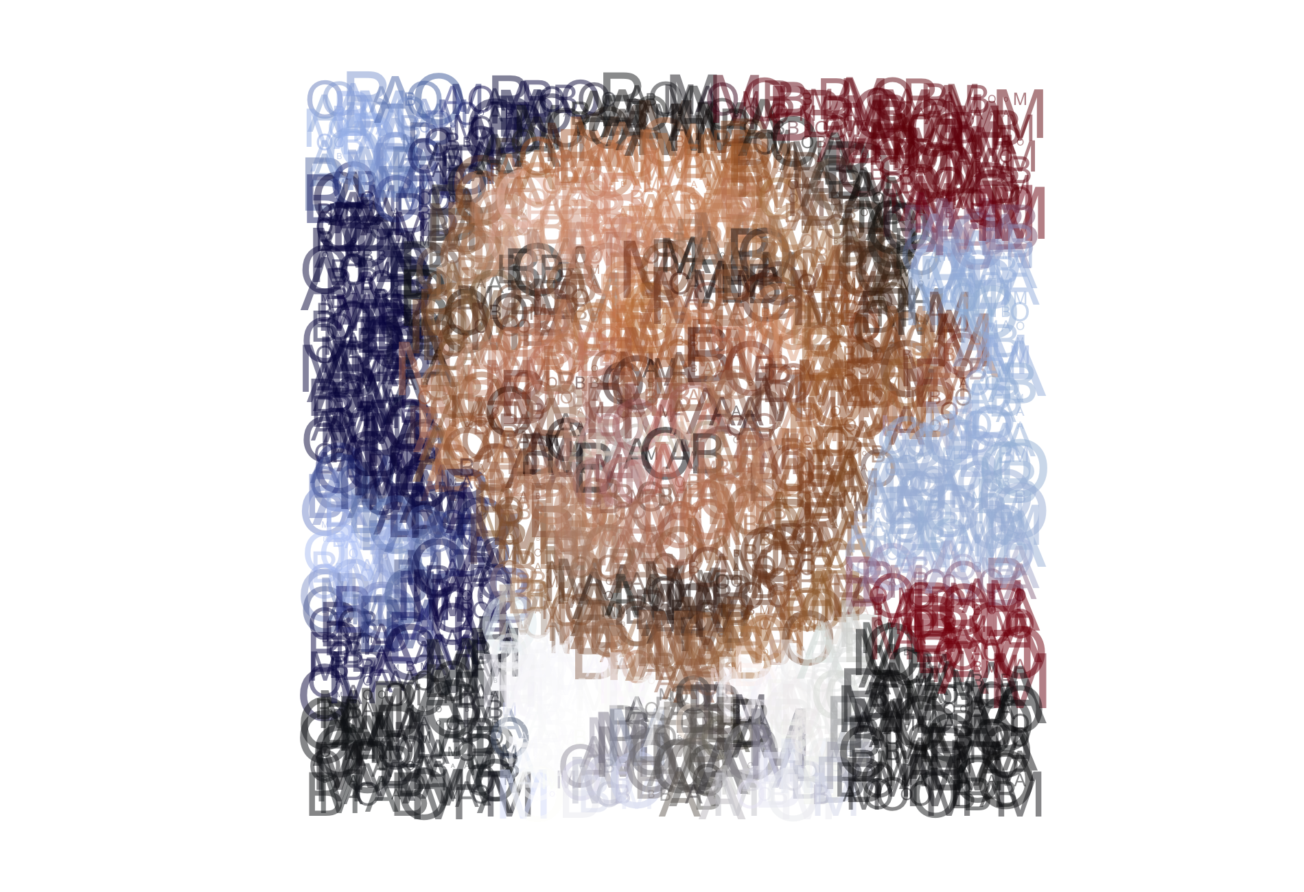
    The code to generate the following image is below.  Enjoy.

    barryO

    
    library(EBImage)
    set.seed(1234)
    #im<-readImage("/Users/gregorymatthews/Dropbox/Rart/queenOfHearts.jpeg")
    #im<-readImage("/Users/gregorymatthews/Desktop/IMG_9074.jpg")
    #im <- readImage("/Users/gregorymatthews/Desktop/guyAlley.jpg")
    im <- readImage("/Users/gregorymatthews/Desktop/barry.png")
    ddd<-dim(im)
    gran<-50
    xxx<-round(seq(1,ddd[1],length=gran))
    yyy<-round(seq(1,ddd[2],length=gran))
    small<-im@.Data[xxx,yyy,]
    ddd<-dim(small)
    
    png("/Users/gregorymatthews/barryO.png",h=13,w=19,unit="in",res=100)
    plot(0,0,frame.plot=F,xlim=c(0,ddd[1]),ylim=c(0,ddd[2]),col="white",asp=1,xaxt='n',yaxt='n',xlab="",ylab="")
    
    for (i in 1:ddd[1]){print(i)
                        for (j in 1:ddd[2]){
                                            points(i,ddd[2]-j,col=rgb(small[i,j,1],small[i,j,2],small[i,j,3],alpha=0.5),pch=sample(c("O","B","A","M"),1),cex=runif(1,0.5,7))
                        }
    }
    
    dev.off()
    

    Cheers.

  • One day at lunch in high school the following exchange took place:

    My friend: “Who plays the blind guy on Star Trek?”

    Me: “It’s LeVar Burton….but you don’t have to take my word for it.”

    You can make this joke relevant again for another generation by donating to my boy LeVar and bringing back Reading Rainbow.

    Also, here is the Reading Rainbow theme music.

    Cheers.


  • Fellow Kaggle champion Mike Lopez has announced that he will be teaching at Skidmore next year! And apparently “investing” his money at the track. Good luck (in both your endeavors), Mike!

    statsbylopez's avatarStatsbyLopez

    This news is about a month old, but I hadn’t updated it on the blog.

    I accepted a position as an assistant professor of statistics at Skidmore College.

    This will be my school year.

    This will be my summer (kind of).

    View original post

  • bbaumer21's avatarExploring Baseball Data with R

    Last time , we learned how to download MLBAM GameDay data using the openWAR package. Specifically, we downloaded data from a single game and created some simple summaries.

    Most often, we’ll be interested in investigated data from many games. The function getData() will download data over any time interval in which you are interested. Let’s figure out how many home runs were hit on May 14th, 2013.

    Visualizing the data

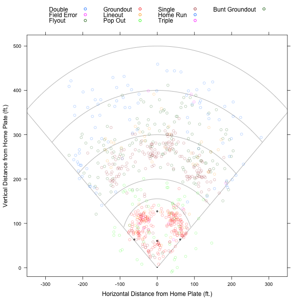
    One nice aspect of the MLBAM data is that it contains an (x,y)-coordinate indicated the location of each batted ball hit into play. getData() returns a data.frame of class GameDayPlays. We have written plot.GameDayPlays() function for visualizing hit location data with a generic field overlaid.

    plot_example

    Note that we have done some of the work to normalize the coordinates provided by MLBAM – though there is still more to be done.

    Modeling

    In order to compute openWAR, we need…

    View original post 570 more words

  • statsbylopez's avatarStatsbyLopez

    Three NHL Game 7’s are scheduled for tonight, so I figured I’d run some Game 7 numbers.

    For this analysis, I used both numbers via AC Thomas’ nhlscrapr package (provided by Thomas himself), and also penalty data that I collected a few years back, summarized in a paper here, a recent article here, and published in International Journal of Sport Finance.

    What’s different about Game 7’s?

    For starters, there are far fewer penalties.

    On average, teams combine for about 9.4 penalties (excluding matching majors) in playoff Game’s 1 through 6, but just 7.0 in Game 7s. This could be the result of changes in style of play, or due to referees being less inclined to assert themselves into the game.

    In terms of win percentage, going back to 2002, home games have won 57% of Game’s 1 through 6, and 52% of Game 7s. Here’s a chart…

    View original post 275 more words

  • statsbylopez's avatarStatsbyLopez

    Momentum does not exist !

    Yes it does!

    No it doesn’t!

    Yes it does!

    Actually, it both exists and doesn’t exist simultaneously!

    Perhaps Rocco Mediate sums it up this debate best, saying 

    “As any athlete knows, momentum is the most unstoppable force in sports. The only way to stop it is if you get in your own way, start making stupid mistakes, or stop believing in yourself.”

    Okay then.

    What to make of all of this? What is the best research that has been done?

    Quantifying momentum is a difficult and arduous task for any researcher, the naive of whom (such as coaches and media members) use anecdotal evidence to drive discourse. Alternatively, there can also be a tendency to use arbitrary cutpoints (i.e., the last five games, or the last 10 plays) when describing momentum, which is also less than ideal.

    Before I try to quantify momentum, I…

    View original post 984 more words

  • With the NBA playoffs now in full swing and 2014 already looking like one of the most entertaining postseasons in recent memory, many basketball fans are focused squarely on the best teams in the league. But for those of us who love the college game, follow teams that didn’t make the playoffs, or simply enjoy all things NBA, it’s also time to start giving a serious look at the upcoming NBA draft, which just might feature the deepest pool of young talent we’ve seen in a decade.

    In analyzing players in the draft, people have a tendency to focus on two main things: which teams the players fit with and which NBA stars it’s easiest to compare the players to. However, at this stage, both of these ideas offer false and/or incomplete evaluations of the incoming players. Comparisons to NBA stars are often hasty and result in unfair expectations. Also, pairing players with teams is somewhat pointless when we don’t even know for sure which teams will be drafting in which spots! So instead of looking too far ahead, here’s a look at how the top three prospects compared to recent rookies coming into the league, from a statistical standpoint.

    Andrew Wiggins

    Viewed by many analysts and fans alike as the biggest talent to enter the NBA Draft since Lebron James, Andrew Wiggins has slipped a bit over the course of the season. In his one year at Kansas, Wiggins didn’t quite dominate the college ranks the way many expected. Although his potential remains enormous, he’s considered by some to be less “NBA-ready” than fellow top prospects like Jabari Parker. But which recent rookie offers the best glimpse of what we might expect from Wiggins? Here’s an eerily close player comparison, courtesy of Sports-Reference:

      • Player A: 17.1 ppg, 5.9 rpg, 1.5 apg, 44.8 FG%, 34.1 3p%


      • Player B: 17.1 ppg, 5.2 rpg, 1.1 apg, 44 FG%, 35.8 3p%


    By the look of those stat lines, Wiggins may not be as unique as we all assumed for a player coming out of college! Player A is Andrew Wiggins (6’8, 200 lbs) in his first and final season at Kansas, and Player B is Harrison Barnes (6’8, 215 lbs) in his last season at North Carolina. Now, Barnes has become a very strong role player for the Golden State Warriors and is even in the midst of helping them through a grueling series against the Clippers. In fact, according to online sports site/betting platform Betfair, the Warriors now have a 6/4 shot of winning this series (a better chance than when the series started). It goes without saying that his 10.5 ppg during the series have been an enormous contribution.

    Overall, however, given that he too was once called the best prospect since Lebron James, Barnes’s career to this point has been mildly disappointing. It’s also fair to note that the stat line provided for Barnes came in his sophomore year, indicating Wiggins was better earlier than Barnes. But given similar levels of competition in college, in the Big 12 and ACC, these are very similar stat lines. Throw in similar sizes, similar positioning (though Wiggins is more of a 2/3 combo, and Barnes perhaps more of a 3/4), and reliance on strong shooting and exceptional athleticism, and Barnes may be a player to watch when projecting Wiggins.

    Jabari Parker

    Right alongside Wiggins as a top prospect is Duke’s Jabari Parker, a Wooden Award finalist who unquestionably had the strongest season among the freshmen in the draft. Parker is viewed as a once-in-a-generation offensive talent who will need to improve on his defense and likely get in better shape. However, people have gotten so caught up in comparing him to Paul Pierce and Carmelo Anthony that there’s virtually no comparison out there to a recent rookie. So how about this one:

      • Player A: 17.5 ppg, 9.2 rpg, 1.2 apg, 51.9 FG%, 40.0 3p%


      • Player B: 19.1 ppg, 8.7 rpg, 1.2 apg, 47.3 FG%, 35.8 3p%


    In this instance, Player A is Jared Sullinger (6’9, 265 lbs) in his final season at Ohio State before becoming a forward for the Boston Celtics, and Player B is Jabari Parker (6’8, 235 lbs) in his lone season at Duke. If this doesn’t seem like as strong a comparison as the Wiggins-Barnes one, it’s because it isn’t, and that’s a positive indication for Parker. Sullinger has been good in the NBA, but he’s a role player—Parker has star potential. Sullinger compiled this stat line as a sophomore and the only real star on his college team, whereas Parker did it playing largely out of position on a Duke team loaded with offensive weapons. The 3p% numbers are skewed somewhat as well, given that Sullinger shot only 40 three pointers that year, and Parker put up 106 at Duke. In this case, it seems as if NBA player comparisons may be more appropriate, because Parker is simply unlike any player to come out of college in recent years.

    Joel Embiid

    The lanky Kansas center might be the trickiest prospect of all to project, because analysts are relying on his potential as much has his proven game. If he meets that potential, many are seeing Embiid as something similar to a Hakeem Olajuwon talent, which is high praise to say the least. But we’ve seen outlandish predictions for tall, coordinated shot blockers with “raw talent” before, and they’re often dubious. However, here’s a player comparison that gives the support for Embiid as a top pick some sturdier legs:

      • Player A: 10.0 ppg, 7.6 rpg, 0.4 apg, 2.7 blk, 53.8 FG%


      • Player B: 11.2 ppg, 8.1 rpg, 1.4 apg, 2.6 blk, 62.6 FG%


    Player A is current Detroit Pistons standout Andre Drummond (6’10, 270 lbs) in his only season at Connecticut, and Player B is Embiid (7’0, 250). Now, these two are very different players, with Drummond relying on his heftier body as the foundation of a more powerful game, and Embiid playing with more touch. Yet against relatively similar levels of competition in the Big East (before it was broken up) and Big 12 respectively, Drummond and Embiid put up similar stats. Embiid did it after not starting the first half of the season, and while dealing with a back injury and a more talented roster of teammates.

    Given Drummond’s early success, this is an exciting indication for Embiid, though again, the two play very differently on the court. CBS Sports recently profiled Embiid as arguably the best center prospect in a decade. However, he is still somewhat raw, he doesn’t have the playing experience of most prospects and his back injury could be cause for concern. If he lives up to potential, though, we’ll see that Embiid is more than just another tall, long project.


  • …and we won.

    statsbylopez's avatarStatsbyLopez

    The website Kaggle sponsored a March Machine Learning Mania contest over the last few months, which involved picking probabilities for every hypothetical NCAA 2014 tournament game.

    Points were awarded, or taken away, given how well each submissions’ probabilities fared, relative to everyone else in the pool (for my statistics-oriented readers, it used the loss function from logistic regression). So, if you picked Florida over Albany with probability 0.80, while Florida won, you would’ve lost ground because the majority of entries had the Gators winning with roughly a 95% probability. Meanwhile, if you picked Ohio State over Dayton with probability 0.55, the Dayton win would’ve helped your entry out, with most folks having OSU as a roughly 80% favorite.

    Kaggle was kind enough to release histograms of the picks for all submissions, like these ones for the Elite 8 games here (alongside our eventual submissions):

    Image

    For example, in the top left, the average…

    View original post 352 more words

  • Big news!  I have accepted an assistant professor position in the Department of Mathematics at Loyola University Chicago.  Everything is now official and me, my wife, and the dogs will be moving to Chicago in August.

    Cheers!