Stats in the Wild

I’m currently attending the 2011 ENAR spring meeting in Miami.  I arrived Sunday night an presented a poster at the opening poster presentation session.  On Monday, I attended two sessions in the afternoon: the survival analysis section and, later, the policy section.

In the policy section, I saw a presentation entitled “Issues in the use of survival analysis to estimate damages in equal employment cases” by Qing Pan and Jooseph L. Gaswirth, which has been published in the journal Law, Probability, and Risk in the March 2009 issue.  The presentation was two-fold: First they presented some basic methods for determining whether or not discrimination had taken place.  In this case (age discrimination),  it was fairly evident that the infraction has occurred.  Second, the authors presented how to assess the compensation that should be awarded to the parties which had been discriminated against.  In order to do so, they applied survival analysis techniques to estimate how long someone would have worked at the company if they had been employed.  Very interesting stuff.

Along the same legal lines, I happened to pick up a book called “A Very Short Introduction to Statistics” by David J. Hand.  While I was flipping through it I came across a section about a woman named Sally Clark.  She was a woman who had two children, both of whom died within the first 11 weeks of their respective lives.  Subsequently, she was charged with murder as it seemed suspicious that TWO of her children had both died so young.  During the trial, Professor Sir Roy Meadow, (famous for proposing the theory of Munchausen Syndrome by Proxy (MSbP)) claimed that the chances of two of her babies dying in this fashion totally by chance was 73,000,000:1.  At those odds, I suppose you would have to convict the person.  However, his method for arriving at this number was flawed.  The Royal Statistics Society issued a statement that began “In the recent highly-publicised case of R v. Sally Clark, a medical expert witness drew on published studies to obtain a figure for the frequency of sudden infant death syndrome (SIDS, or “cot death”) in families having some of the characteristics of the defendant’s family. He went on to square this figure to obtain a value of 1 in 73 million for the frequency of two cases of SIDS in such a family.”  (Read the whole statement here.)  The way I feel about this can be summed up by some comments my friend (a lawyer) made when I emailed him about this case: “That’s wild that that happened in 1999. I figured it would be like
1899.”

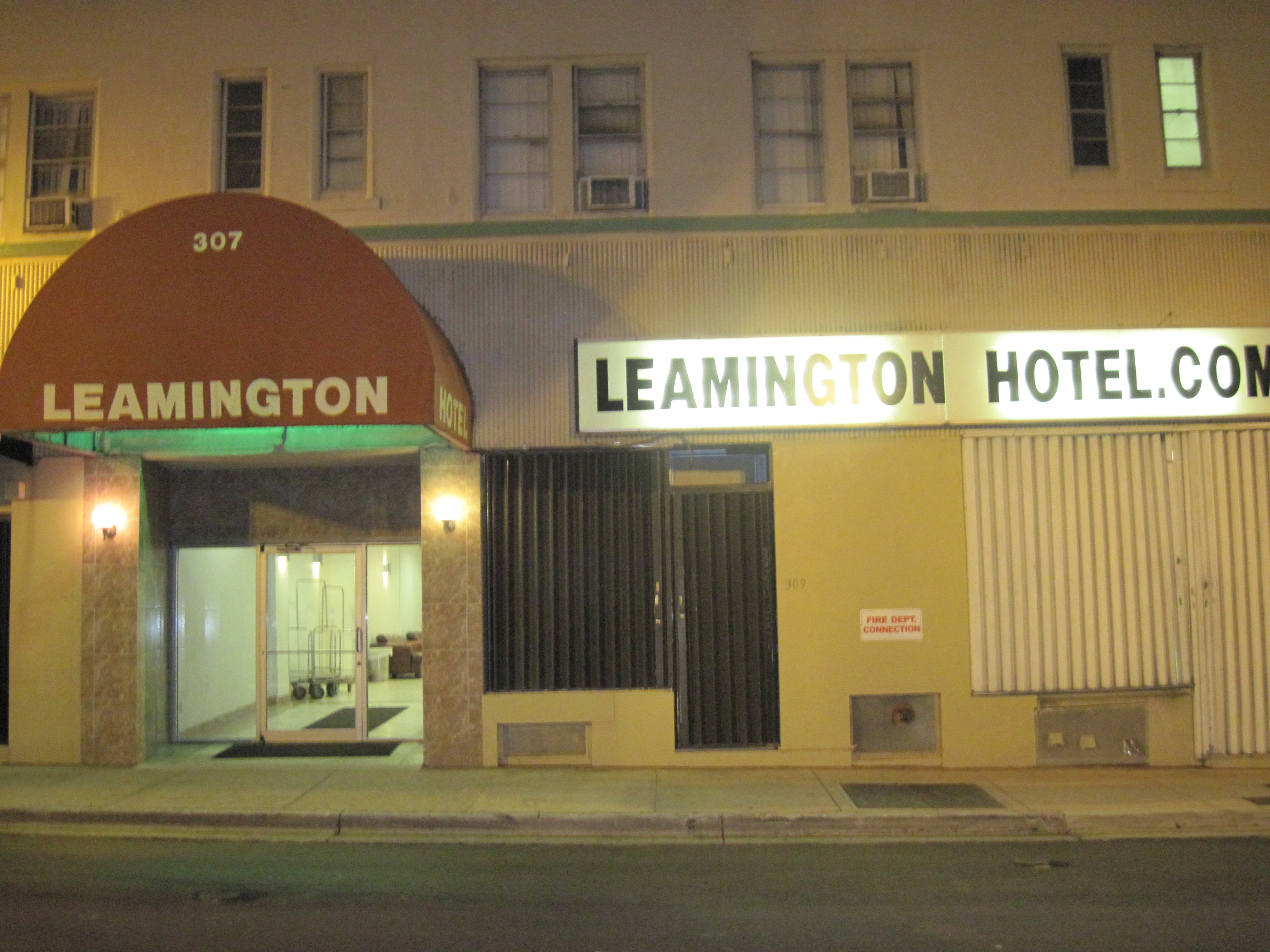
So anyway, I am now sitting in my hotel room at the Leamington (students can’t afford the Hyatt).  I’ll leave you with a picture of the hotel I am staying at.  I can’t wait to get a job.

Cheers.

Here are the StatsInTheWild rankings of the NFL teams after Week 10.
Rank Teams Wins
1 NewEngland 7
2 Atlanta 7
3 NYJets 7
4 Pittsburgh 6
5 Baltimore 6
6 Miami 5
7 Philadelphia 6
8 NewOrleans 6
9 TampaBay 6
10 GreenBay 6
11 Indianapolis 6
12 Tennessee 5
13 Cleveland 3
14 NYGiants 6
15 Chicago 6
16 Jacksonville 5
17 KansasCity 5
18 Oakland 5
19 Seattle 5
20 SanDiego 4
21 Houston 4
22 Washington 4
23 Denver 3
24 Minnesota 3
25 Cincinnati 2
26 Arizona 3
27 StLouis 4
28 SanFrancisco 3
29 Dallas 2
30 Detroit 2
31 Buffalo 1
32 Carolina 1

The two teams that pop out are the Giants and the Browns. The Browns are 3-6 with wins over the Bengals, Saints, and Patriots. Their losses are to Tampa Bay, Kansas City, Baltimore, Atlanta, Pittsburgh, and the Jets. Those teams average 6.33 wins each and all hold at least a share of the lead in their respective division.

The Giants have losses to Indianapolis, Tennessee, and Dallas. They have beaten Carolina, Chicago, Houston, Detroit, Dallas, and Seattle. The six teams they have beaten average only 3.33 wins. A vast difference in schedule.

I also wrote some code to simulate the rest of the NFL season based on what has already happened. So I used the games that have already occurred as data for a model (a very simply model). This model predicts the probability of a win for a given team. Then the rest of the season is simulated 5000 times based on the estimated probabilities of winning a game.
Here are the results of that:

Probability that a team wins its division:
Division Winners:
AFCEast
Miami NewEngland NYJets
0.0080 0.6004 0.3916

AFC North
Baltimore Cleveland Pittsburgh
0.4712 0.0004 0.5284

AFC South
Houston Indianapolis Jacksonville Tennessee
0.0020 0.6158 0.1058 0.2764

AFC West
Denver KansasCity Oakland SanDiego
0.0450 0.5646 0.2138 0.1766

NFC East
NYGiants Philadelphia Washington
0.1850 0.8118 0.0032

NFC North
Chicago GreenBay Minnesota
0.2066 0.7886 0.0048

NFC South
Atlanta NewOrleans TampaBay
0.9150 0.0432 0.0418

NFC West
Arizona SanFrancisco Seattle StLouis
0.1726 0.0374 0.6958 0.0942

Conference Champions:
AFC
Baltimore Cleveland Indianapolis Jacksonville KansasCity Miami
0.1524 0.0002 0.0378 0.0010 0.0008 0.0078
NewEngland NYJets Oakland Pittsburgh Tennessee
0.3418 0.1844 0.0138 0.2586 0.0014

NFC
Atlanta Chicago GreenBay NewOrleans NYGiants Philadelphia
0.5882 0.0280 0.0484 0.0556 0.0084 0.2106
Seattle TampaBay
0.0156 0.0452

Super Bowl Champion:

Atlanta Baltimore Chicago GreenBay Indianapolis KansasCity
0.3112 0.0862 0.0040 0.0126 0.0094 0.0002
Miami NewEngland NewOrleans NYGiants NYJets Oakland
0.0032 0.2154 0.0154 0.0016 0.1068 0.0022
Philadelphia Pittsburgh Seattle TampaBay Tennessee
0.0640 0.1522 0.0016 0.0134 0.0006

So, right now SITW is predicting a Atlanta Falcons – New England Patriots Superbowl with Atlanta winning.

Cheers.

So I’m in a poker league. We play three out of four Thursday nights in a month for a total of fifteen events in a season. Each event you earn a certain number of points. You’re 10 best finishes based on points out of the fifteen events are counted. After the grueling fifteen week season, there is a finale where you start with an amount of chips proportional to the number of points you earned during the season. Anyway, another player (Shaun) and I took over the scoring for the league this season. Our scoring system is pretty basic (50 points for showing up, 50 points for everyone you beat, 600-300-150-75 bonus for cashing (finishing top 4)). On top of this I’ve devised a fairly reasonable ranking system separate from the points based on your average finish and how many events you have played. One criticism of my ranking system is that I’m not accounting for the strength of the field, I’m just looking at average percentile of finish.

So I usually car pool to and from events with Shaun and we’ve been talking about ranking systems. Last night he mentioned that he had been doing some research on how Xbox live does their rankings. Each player has some level of ability and an uncertainty associated with their skill level. After each game players rankings, skill level and uncertainty, are updated. He described it a little bit more, and I mentioned that it sounded Bayesian to me. Turns out it is!

Here is an introduction to the TureSkill ranking system and here is a more detailed description. For those of you who are interested in all the details, here is the paper “TrueSkill(TM): A Bayesian Skill Rating System” where they propose the system.

Cheers.

P.S. A big SITW congratulations to James T. O’Connor of Belchertown, MA for passing the CT bar exam.

P.P.S. I finished second in the regular season last year, but won the finale. This year I was briefly in first place until last night. I am now in second place by 150 points with 4 events to play.

I’m teaching my first class this fall, and I’ve been preparing my notes for class this past week. I wanted to use keno as an example of how to compute probabilities. So I was computing some probabilities and checking them against the posted “odds” on masslottery.com. I couldn’t get my computed odds to match with what the lottery had posted, which led to a brief period of panic that I wasn’t qualified to be teaching this class. Turns out, I’m not computing anything wrong. It’s just that what the lottery is calling “odds” are actually probabilities. Take a look again at masslottery.com and look at the posted odds for a one spot game. For the one spot game they say that the odds are 1:4. This is incorrect. The probability of winning this one spot game is , which would make the odds of winning . Likewise, the odds against winning are 3:1. Generally, if the probability of an event is p, the odds of this even occuring are .

So what the lottery is referring to as odds are actually probabilities of winning. They actually get this correct that the bottom where they say “Probability of winning a prize in this game = 1:4.00”. The mistake is that they aren’t making any distinction between the probability of winning and the odds of winning when, in fact, these are different.

Cheers.