• It’s true. I am doing terrible in the NFL this year. But so is basically everyone else.

    statsbylopez's avatarStatsbyLopez

    It’s still relatively early in the NFL season, but signs point to this being one of the worst seasons ever for simulation & statistics based predictors of game results. In fact, having followed several websites for the last few years, this is by far the worst I can remember each one doing as far as accuracy is concerned.

    Here, I summarize results through week 7.

    Football Outsiders (FO) : These guys have pretty much set the standard for NFL statistical analyses, as demonstrated by their preseason almanacs, appearances across the media, and downloadable spreadsheets with all sorts of good information. In their first five years of picking games against the spread (ATS), from 2008 to 2012, FO finished with yearly success rates of 53.7%, 51.2%, 56.1%, 52.0%, and 57.8%, respectively. There’s no public access for historical picks, but I’ve followed along and these numbers are 100% trustworthy.

    This Fall, however…

    View original post 606 more words

  • It’s true. I am doing terrible in the NFL this year. But so is basically everyone else.

    statsbylopez's avatarStatsbyLopez

    It’s still relatively early in the NFL season, but signs point to this being one of the worst seasons ever for simulation & statistics based predictors of game results. In fact, having followed several websites for the last few years, this is by far the worst I can remember each one doing as far as accuracy is concerned.

    Here, I summarize results through week 7.

    Football Outsiders (FO) : These guys have pretty much set the standard for NFL statistical analyses, as demonstrated by their preseason almanacs, appearances across the media, and downloadable spreadsheets with all sorts of good information. In their first five years of picking games against the spread (ATS), from 2008 to 2012, FO finished with yearly success rates of 53.7%, 51.2%, 56.1%, 52.0%, and 57.8%, respectively. There’s no public access for historical picks, but I’ve followed along and these numbers are 100% trustworthy.

    This Fall, however…

    View original post 606 more words

  • Updated: October 24, 2013

    Pro: The rankings are based on how a team performs and accounts for how many points they would be expected to score based on their statistical output such as rushing yards, passing yards, etc.  This ranking considers past seasons statistics with heavier weights placed on games that are more recent.  This ranking is the more predictive of the two.

    Retro: This ranking only considers strength of schedule and the actual outcome of games in 2013.  This is a ranking of who actually has had the best season.

    SOS: Is strength of schedule.

     
    Team Pro Retro W L sos
    Kansas City 1 1 7 0 2
    Denver 3 2 6 1 23
    Seattle 2 3 6 1 14
    New Orleans 7 4 5 1 6
    Indianapolis 6 5 5 2 19
    San Francisco 8 6 5 2 18
    Green Bay 5 7 4 2 16
    Dallas 9 8 4 3 1
    San Diego 11 9 4 3 28
    Cincinnati 14 10 5 2 12
    New England 10 11 5 2 15
    Detroit 12 12 4 3 17
    Carolina 4 13 3 3 13
    Miami 16 14 3 3 5
    Chicago 21 15 4 3 9
    Tennessee 15 16 3 4 21
    Arizona 17 17 3 4 25
    Baltimore 13 18 3 4 11
    Philadelphia 18 19 3 4 3
    Oakland 23 20 2 4 26
    Atlanta 19 21 2 4 20
    St. Louis 25 22 3 4 29
    Cleveland 24 23 3 4 10
    Washington 22 24 2 4 24
    NY Jets 26 25 4 3 8
    Buffalo 20 26 3 4 4
    Pittsburgh 28 27 2 4 7
    Houston 27 28 2 5 32
    NY Giants 31 29 1 6 31
    Jacksonville 32 30 0 7 30
    Minnesota 30 31 1 5 22
    Tampa Bay 29 32 0 6 27
  • The Red Sox and Cardinals meeting in the Fall Classic represents the top run differentials in each league squaring off. Baseball statheads should feel the warm glow of empiricism peeking through, especially after last year when we had to hear from some about the overrating of run differential. Why is it at all controversial to say that the team largest difference between runs scored and runs allowed over 162 games? Is that a radical notion? I think part of it is the basic notion that most people don’t understand randomness (or “luck” or “fortuosity” or “midichlorians” or whatever you want to call it) and that even in a large sample of 162 games, you can have smaller sub-samples (like the Orioles’ 38 one-run games last season, in which they went an insane 29-9) where randomness can take over, and then the whole sample ends up a bit screwy.

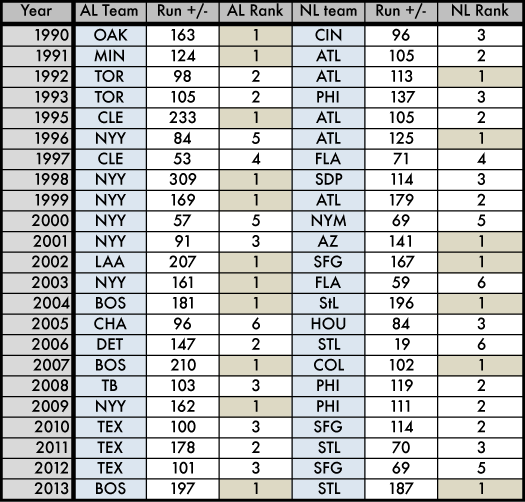
    But I digress, the Boston Red Sox scored 197 more runs than they allowed, more than any other AL team and the St. Louis Cardinals scored 187 more runs than they allowed, more than any other NL team. So we are poised to see the Pythagorean Pennant winners face off. How does this compare to previous years’ match-ups? I’m glad I asked myself, because I spent some time compiling the run differentials of each league’s WS representatives, plus the overall WS run differential, as well as each teams’ rank in their respective leagues since 1990 (remember that there was no World Series in 1994.) I highlighted the teams who lead their league in run differential in gold, cause they’re special, you know?
    graph
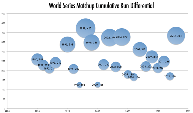
    This doesn’t mean all that much, I suppose. But it’s hasn’t been exactly common for each league’s top run +/- team to get to the WS to square of, so I thought I’d look at some stuff.  And also, I made a couple little bubble charts to visualize the run diffs of the respective teams. Of course, the cumulative run differential means only so much. The best cumulative run differential was from 1998, but that was the historically great 1998 Yankees team, who have the best run differential in the last 24 seasons (the also historically great 2001 Mariners are second best, with 301 to the Yanks’ 309. After them, it’s a long fall to third place). Because of this, I made a second graph that plots the difference (the run differential is NL team minus AL team, so negative values represent a matchup favoring the AL). With this, you can see just how much better the Yanks’ run differential was than the Padres, and the Padres had the third best in the NL in 98. In this chart, I also put the WS numbers in red when the team with the better run differential lost. (click to enlarge, please. )
    Image
    Image
    Here are some interesting facts I gleaned from this exercise- The Red Sox have played in three WS since 1990 and each time they’ve had the best run differential in the AL* have faced the best run differential from the NL. In fact, there have been four WS with the best vs best, and the only non-Red Sox one is the 2002 Series between the Angels and Giants. The worst WS in terms of total run differential was 1997, where Florida and Cleveland had a cumulative run differential of +124 (compare that with the best team in each league, the Yankees, who had a +210, and Atlanta, at +203). The worst in terms of rankings (and barely missed cumulative), was the 2000 Subway Series, where the Yankees and Mets were each the fifth best in their leagues, and the had a cumulative total of +126 (Giants had the best in the NL at +178 and the White Sox were the AL’s best at +138.) The team with better run differential has lost 13 of the 22 series (with 2013 outstanding, obviously). What does that mean?  A seven game series features a lot of that randomness. The Marlins were 102 runs were than the Yankees in 2003, and won in six. The 2006 Cardinals were a whooping 128 runs worse than the Tigers in 2006 (that’s right, Detroit managed to outdo their OPPONENT’s run differential by more than the cumulative totals of either the 1997 series or 2000 series teams) and the Cards won in five.

    * One fact that always seems to be left out when narratives are being created about the 2004 Red Sox is that they led the AL in run differential and it was about as close as Reagan vs Mondale. The Red Sox scored 181 more runs than they allowed. The second place AL team was the Angels, at +102, third was the Yankees at +89. The Red Sox’ expected record  was 98 wins, same as their actual record. It was the 2004 Yankees whose record was grossly out of tune with their expected win-loss, as they won 101 games but were expected to win only 89 (which actually would have placed them behind the A’s for the Wild Card). It wasn’t that the Red Sox were scrappy and overcame obstacles, it was more that they were the much better team, best in the AL, and the Yankees’ magic dust finally wore out. It’s not as fun of a narrative, but it’s got a better empirical basis. Of course, it still doesn’t explain why the Yankees never bunted on Curt Schilling and his bloody sock, but that’s strategy, not empiricism.
    What we can say is that the 2013 World Series features two teams whose run differential is very close. We’ve also had 10 World Series since 1990 (including this one) that features teams within 20 runs of each other. You cannot predict the outcomes of these matchups. The old adage that “good pitching beats good hitting” is literally meaningless. Max Scherzer and Justin Verlander did not trump the  Red Sox and their MLB-best offense, and Zach Greinke and Clayton Kershaw did not silence the NL-best Cardinals offense. Anything can happen in a short series, and seven games is pretty short in baseball. But 162 is anything but short, and we do know that based on a whole season’s worth of data, in 2013, we get to see the two best possible teams playing each other. Let’s hope it’s worth watching.
  • I really enjoyed the below comment from this Deadspin article:

    This sir, is exactly how I feel. I’m a journalism student and my professors hate Bill Simmons. Not because he isn’t a talent journalist, but he hasn’t been a journalist for the last 5 years and yet writes douchebag seriousness on his “Grantland” website that many take as gospel. I like Katie Baker and some of the others on Grantland, but Simmons and O’Reilly just need to get locked in a room by themselves and see who’s ego wins. At least then, we would only have one profound douche in sports media.

    Cheers!

  • I tweeted earlier today expressing sketicism about an article I read on the Regressing section of Deadspin about west coast football teams travelling to the east coast. I thought that when I had some time tonight, I’d downlaod the data and explore the question myself, but it looks like Mike Lopez (@statsbylopez) beat me to it. And my skepticism may have been warranted.

    Cheers.

    statsbylopez's avatarStatsbyLopez

    “There are lies, damned lies, and statistics”-Mark Twain

    There was an interesting post at sportsinsights.com earlier today, which looked at the performances of West Coast NFL teams based on game location. The authors hypothesize that “NFL West Coast teams traveling east suffer declines in performance.”

    It’s an interesting idea, and, if true, could make the NFL re-think scheduling, which often requires teams to travel thousands of miles on consecutive weekends. Moreover, I liked how the authors looked at team performance against the spread, in contrast to this article at Advanced NFL Stats, which simply looked at team performance, and thus was not able to account for difference’s in the abilities between teams on different coasts.

    The topic was interesting enough that it was look at by more than 12,000 viewers (as of 4:52, Friday) when linked by Deadspin.

    Further, the results of the Sports Insights study are interesting…

    View original post 568 more words

  • 2013-Week-6-Playoff-Probs

    The Bears seem to be trying to echo last year, where they spent most of the season as the NFC North’s favorites until they ceded ground to the Packers. Meanwhile, the Saints didn’t take too much of a hit from that heartbreaking last-minute loss to the Pats, while the Jets did. And, I guess, better luck next year Chargers and Raiders (sorry, Terrelle). Click the image to see this baby in its full-sized beauty.

  •  
     Rank Team Record
    1 MISSOURI 6-0
    2 FLORIDA STATE 5-0
    3 CLEMSON 6-0
    4 OREGON 6-0
    5 STANFORD 5-1
    6 GEORGIA 4-2
    7 OHIO STATE 6-0
    8 MIAMI-FLORIDA 5-0
    9 ARIZONA STATE 4-2
    10 ALABAMA 6-0
    11 SO CAROLINA 5-1
    12 UTAH 4-2
    13 LSU 6-1
    14 FLORIDA 4-2
    15 WASHINGTON 4-2
    16 BAYLOR 5-0
    17 MICHIGAN STATE 5-1
    18 BYU 4-2
    19 UCLA 5-0
    20 VIRGINIA TECH 6-1
    21 TEXAS A&M 5-1
    22 AUBURN 5-1
    23 OREGON STATE 5-1
    24 LOUISVILLE 6-0
    25 USC 4-2

    Full Rankings

    Cheers.


  • Introduction

    I recently wrote an article about Football Outsiders flawed argument about NFL place kickers. The Football Outsider’s people responded, and I wrote a rebuttal here.  The original piece from Football Outsiders that sparked my interest in this topic is below:

    Field-goal percentage is almost entirely random from season to season, while kickoff distance is one of the most consistent statistics in football.

    This theory, which originally appeared in the New York Times in October 2006, is one of our most controversial, but it is hard to argue against the evidence. Measuring every kicker from 1999 to 2006 who had at least ten field goal attempts in each of two consecutive years, the year-to-year correlation coefficient for field-goal percentage was an insignificant .05. Mike Vanderjagt didn’t miss a single field goal in 2003, but his percentage was a below-average 74 percent the year before and 80 percent the year after. Adam Vinatieri has long been considered the best kicker in the game.But even he had never enjoyed two straight seasons with accuracy better than the NFL average of 85 percent until 2011, when he followed up his 26-for-28 2010 campaign by going 23-for-27 (85.2 percent).

    On the other hand, the year-to-year correlation coefficient for kickoff distance, over the same period as our measurement of field-goal percentage and with the same minimum of ten kicks per year, is .61. The same players consistently lead the league in kickoff distance, particularly Billy Cundiff, Olindo Mare, and Stephen Gostkowski.

    “NFL Kickers Are Judged on the Wrong Criteria,” New York Times, November 12, 2006

    Pro Football Prospectus 2007, Arizona chapter

    The basic gist of the NY Times article is that kickers are inconsistent from year to year and the argument is based solely on field goal percentage made.  There are two major flaws that I perceive in this argument.  The first is that they don’t control for any covariates that would affect variability such as the most obvious predictor, distance of the field goal attempt.  (I see that Football Outsiders is controlling for length of kick when they are calculating DVOA, but I’m still not convinced they controlled for distance when making the statement that “Field-goal percentage is almost entirely random from season to season”.)  The second is that I don’t think FO is making a distinction between the actual percent of field goals made by a given kicker and the probability of a given field goal kicker making a field goal.  For example, let’s say a given kicker kicks 40 field goals per year all from the same distance and the probability of success on every field goal is the same at 0.8.  Here is what ten simulated seasons look like under these conditions:

    rbinom(10,40,0.8)/40
    
    [1] 0.925 0.825 0.875 0.775 0.800 0.825 0.750 0.875 0.700 0.875
    

    You can see that the kicking percentage for this kicker has quite a bit of variability. In their first season they made 92.5% of their kicks and then in their ninth year they made only 70% of their kicks. But their ability over these ten years was exactly the same. The differences in the field goal kicking percentages is completely due to random chance even though their ability was constant. So, we aren’t so interested in answering the question of whether or not kickers field goal percentages change from year you year; That’s essentially a meaningless question. We’re interested in whether or not the probability that a kicker will make a field goal, their ability, changes from year to year.

    So I agree completely with the statement that “Field-goal percentage is almost entirely random from season to season”. But again that doesn’t really mean anything. The question that I think we’re really interested in here is “Does the ability of a place kicker change significantly from year you year?”  It seems like FO was trying to answer this question by comparing field-goal percentages, but they really should have been asking whether the probability of making a kick for a given kicker varies from year to year.

    I’m going to explore this using mixed effects logistic regression modeling to look for evidence of variability in kickers abilities from year to year.

    Analysis

    To begin this analysis I needed to collect some data. I collected data from www.pro-football-reference.com in their box scores.  My full scraping code can be seen at the end of this post in the appendix or viewed on github here.

    summary(kick.dat$yards)
    #Min. 1st Qu. Median Mean 3rd Qu. Max.
    #18.00 28.00 37.00 36.37 45.00 76.00
    table(kick.dat$good)
    #0 1
    #1610 7273
    table(kick.dat$year)
    ##2011 2010 2009 2008 2007 2006 2005 2004 2003
    ##1053 997 968 1038 993 990 986 892 966
    tapply(kick.dat$good,kick.dat$year,mean)
    ##2011 2010 2009 2008 2007 2006 2005 2004 2003
    ##0.8309592 0.8224674 0.8057851 0.8448940 0.8257805 0.8202020 0.8103448 0.8082960 0.7960663
    

    I collected data from 2003-2004 through 2011-2012 season. The median length of field goal attempt over this period of time was 37 yards. 8,883 total field goals were attempted (987 per year on average) of which 81.88% of attempted field goals over this period of time were converted. It also appears field goal success percentage is trending upwards over the course of these 9 years. This could easily be explained if the mean length of field goals was getting smaller over the course of these nine years, but based on the box plot below, it does not appear that there is a trend of field goal distance getting shorter on average.
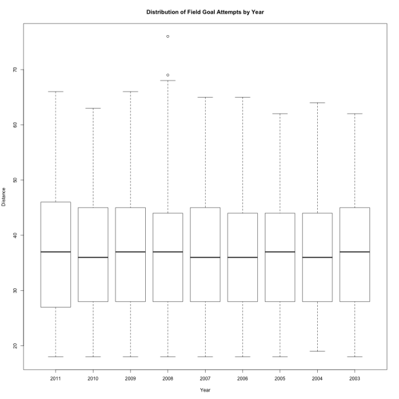
    boxplot by year

    Models

    I built a logistic regression model with the outcome 0/1 for missed/made field goals. I initially included only a fixed for distance of the field goal (actually square root of distance), but after some exploration, I also needed to include a dummy variable for the the year. This means that as a whole for all kickers, the baseline probability of making a field goal is significantly different from season to season. Next, I added a random effect for kicker and another random effect for kicker by year. The first random effect assesses the different abilities of kickers in the NFL and the second random effect assesses the difference in abilities between years for a given kicker. If this second random effect variance estimate is large, that indicates evidence that kickers abilities are actually different from year to year. The output from this model appears below.

    Generalized linear mixed model fit by maximum likelihood ['glmerMod']
    Family: binomial ( logit )
    Formula: good ~ I(yards^0.5) + year + (1 | name) + (1 | name:year)
    Data: kick.dat
    
    AIC       BIC    logLik  deviance
    7237.243  7322.346 -3606.622  7213.243
    
    Random effects:
    Groups    Name        Variance  Std.Dev.
    name:year (Intercept) 8.690e-11 9.322e-06
    name      (Intercept) 4.317e-02 2.078e-01
    Number of obs: 8883, groups: name:year, 352; name, 78
    
    Fixed effects:
    Estimate Std. Error z value Pr(>|z|)
    (Intercept)   9.91805    0.30610   32.40  < 2e-16 ***
    I(yards^0.5) -1.32140    0.04445  -29.73  < 2e-16 ***
    year2010     -0.13349    0.12694   -1.05  0.29297
    year2009     -0.28794    0.12606   -2.28  0.02236 *
    year2008      0.02418    0.12908    0.19  0.85141
    year2007     -0.17933    0.12834   -1.40  0.16232
    year2006     -0.25091    0.12796   -1.96  0.04991 *
    year2005     -0.30528    0.12727   -2.40  0.01646 *
    year2004     -0.31881    0.13116   -2.43  0.01507 *
    year2003     -0.35993    0.12817   -2.81  0.00498 **
    ---
    Signif. codes:  0 ‘***’ 0.001 ‘**’ 0.01 ‘*’ 0.05 ‘.’ 0.1 ‘ ’ 1
    

    Results

    Below is a plot of the probability of making a kick by distance of the kick. Each line represents a different season with the blue curves representing the more recent years 2007-2011 and the red curves are for the seasons 2003-2006. So it looks like, on the whole, kickers in the NFL are getting better (This Sloan paper reaches the same conclusion).

    AllKickersbyYear

    Next let’s look at how much variability there is within kickers between years.  The plot below displays the probability that a fixed kicker will make a kick based on the distance of the field goal when a fixed effect for year is NOT included in the model.    The red and blue lines represent the 5th and 95th percentile of the distribution of the probability for a kicker between years.  This means that there IS variability in the ability of a kicker from year to year when not including a fixed effect of year, but this variability is relatively small. However……

    KickerAndYearNOFEyear

    If a fixed effect of year is included in the model the standard deviation estimate for the random effect of year by kicker is 9.322e-06.  The plot below is the same as the one above, but a fixed effect of year is included here.  The red and blue lines represent the 5th and 95th percentile of the distribution of the probability for a kicker between years.  From this plot, you can see that there is almost no difference within a kicker between years.  This variability is almost entirely explained by the group improvement in all of the kickers in the NFL.

    KickerAndYearFEyearConclusions

    • There is evidence there is considerable variability between the abilities of NFL kickers.
    • The variability that kickers seem to exhibit from year to year does not seem to be within kickers, it seems to be that kickers are getting better from year to year.  When you control for this group improvement there is ALMOST NO detectable variability in the ability of kickers from year to year.
    • Kickers as a whole seem to be getting better over time.  
    • 2008 was an especially good year for kickers.  Almost 84.5% of field goals were made.

    Appendix

    If you are interested in my scraping code you can see it below or on github here.

    library(XML)
    #Define function for getting kicking data
    get.x<-function(date,team){
    	url<-paste0("http://www.pro-football-reference.com/boxscores/",date,"0",team,".htm")
    
    x<-readHTMLTable(url,header=FALSE)$pbp_data
    
    x<-x[x$V1!="",]
    
    x<-as.character(x$V6)
    
    x<-x[!is.na(x)]
    
    out<-x[unlist(gregexpr("field goal",x))>0]
    out}
    
    #get.x('20120930',"atl")
    
    #Getting the data
    month.hash<-list()
    #month.hash[['08']]<-31
    month.hash[['09']]<-30
    month.hash[['10']]<-31
    month.hash[['11']]<-30
    month.hash[['12']]<-31
    month.hash[['01']]<-31
    month.hash[['02']]<-29
    
    #kick.list<-list()
    year<-"2012"
    t.vec<-c("gnb","phi","htx","nor","crd","den","cle","min","tam","chi","nyj","oti","rav","rai","nyg","ram","was","buf","kan","clt","car","sea","mia","sfo","sdg","dal","pit","nwe","jax","atl","det","cin")
    	for (yearmonth in c(paste0(year,c("09","10","11","12")),paste0(as.character((as.numeric(year)+1)),c("01","02")))){
    			#for (yearmonth in c("201109","201110","201111","201112","201201","201202")){
    	month<-substring(yearmonth,5,6)
    for (day in c(paste0("0",c(1:9)),as.character(c(10:month.hash[[month]])))){
    	for (t in t.vec){
    		d<-paste0(yearmonth,day)
    			print(c(year,yearmonth,day,t))
    			tmp<-try(get.x(d,t))
    			print(tmp)
    			if (class(tmp)!="try-error"){kick.list[[year]][[paste0(d,t)]]<-tmp}
    				}
    				}}
    
    make.kick.df<-function(year){
    kick.vec<-c(unlist(kick.list[[year]]))
    #remove '(no play)'
    kick.vec<-kick.vec[unlist(gregexpr('(no play)',kick.vec))<0]
    
    #pull out yardage
    yards.index<-unlist(lapply(gregexpr('[0-9]',kick.vec),min))
    yards<-substring(kick.vec,yards.index,yards.index+1)
    
    #Pull out kicker name
    name<-gsub(" ","",substring(kick.vec,1,yards.index-2))
    
    #Did they make it?
    good<-yards
    good<-0
    good<-(unlist(gregexpr("field goal good",kick.vec))>0)+0
    
    out<-data.frame(name,yards,good,year=year)
    out
    }
    kick.df<-list()
    kick.df[['2012']]<-make.kick.df('2012')
    kick.df[['2011']]<-make.kick.df('2011')
    kick.df[['2010']]<-make.kick.df('2010')
    kick.df[['2009']]<-make.kick.df('2009')
    kick.df[['2008']]<-make.kick.df('2008')
    kick.df[['2007']]<-make.kick.df('2007')
    kick.df[['2006']]<-make.kick.df('2006')
    kick.df[['2005']]<-make.kick.df('2005')
    kick.df[['2004']]<-make.kick.df('2004')
    kick.df[['2003']]<-make.kick.df('2003')
    kick.df[['2002']]<-make.kick.df('2002')
    kick.df[['2001']]<-make.kick.df('2001')
    kick.df[['2000']]<-make.kick.df('2000')
    #save.image("Kick_Database.RData")
    
    kick.dat<-do.call(rbind,kick.df)
    kick.dat$yards<-as.numeric(as.character(kick.dat$yards))
    #write.csv(kick.dat,"kick_dat.csv")
    
  • 2013-Week-5-Playoff-Probs

    Done up stylish-ly, as we did last year. Just in time for them to not actually matter. Thank you, week six.