Here are the StatsInTheWild rankings of the NFL teams after Week 10.
Rank Teams Wins
1 NewEngland 7
2 Atlanta 7
3 NYJets 7
4 Pittsburgh 6
5 Baltimore 6
6 Miami 5
7 Philadelphia 6
8 NewOrleans 6
9 TampaBay 6
10 GreenBay 6
11 Indianapolis 6
12 Tennessee 5
13 Cleveland 3
14 NYGiants 6
15 Chicago 6
16 Jacksonville 5
17 KansasCity 5
18 Oakland 5
19 Seattle 5
20 SanDiego 4
21 Houston 4
22 Washington 4
23 Denver 3
24 Minnesota 3
25 Cincinnati 2
26 Arizona 3
27 StLouis 4
28 SanFrancisco 3
29 Dallas 2
30 Detroit 2
31 Buffalo 1
32 Carolina 1

The two teams that pop out are the Giants and the Browns. The Browns are 3-6 with wins over the Bengals, Saints, and Patriots. Their losses are to Tampa Bay, Kansas City, Baltimore, Atlanta, Pittsburgh, and the Jets. Those teams average 6.33 wins each and all hold at least a share of the lead in their respective division.

The Giants have losses to Indianapolis, Tennessee, and Dallas. They have beaten Carolina, Chicago, Houston, Detroit, Dallas, and Seattle. The six teams they have beaten average only 3.33 wins. A vast difference in schedule.

I also wrote some code to simulate the rest of the NFL season based on what has already happened. So I used the games that have already occurred as data for a model (a very simply model). This model predicts the probability of a win for a given team. Then the rest of the season is simulated 5000 times based on the estimated probabilities of winning a game.
Here are the results of that:

Probability that a team wins its division:
Division Winners:
AFCEast
Miami NewEngland NYJets
0.0080 0.6004 0.3916

AFC North
Baltimore Cleveland Pittsburgh
0.4712 0.0004 0.5284

AFC South
Houston Indianapolis Jacksonville Tennessee
0.0020 0.6158 0.1058 0.2764

AFC West
Denver KansasCity Oakland SanDiego
0.0450 0.5646 0.2138 0.1766

NFC East
NYGiants Philadelphia Washington
0.1850 0.8118 0.0032

NFC North
Chicago GreenBay Minnesota
0.2066 0.7886 0.0048

NFC South
Atlanta NewOrleans TampaBay
0.9150 0.0432 0.0418

NFC West
Arizona SanFrancisco Seattle StLouis
0.1726 0.0374 0.6958 0.0942

Conference Champions:
AFC
Baltimore Cleveland Indianapolis Jacksonville KansasCity Miami
0.1524 0.0002 0.0378 0.0010 0.0008 0.0078
NewEngland NYJets Oakland Pittsburgh Tennessee
0.3418 0.1844 0.0138 0.2586 0.0014

NFC
Atlanta Chicago GreenBay NewOrleans NYGiants Philadelphia
0.5882 0.0280 0.0484 0.0556 0.0084 0.2106
Seattle TampaBay
0.0156 0.0452

Super Bowl Champion:

Atlanta Baltimore Chicago GreenBay Indianapolis KansasCity
0.3112 0.0862 0.0040 0.0126 0.0094 0.0002
Miami NewEngland NewOrleans NYGiants NYJets Oakland
0.0032 0.2154 0.0154 0.0016 0.1068 0.0022
Philadelphia Pittsburgh Seattle TampaBay Tennessee
0.0640 0.1522 0.0016 0.0134 0.0006

So, right now SITW is predicting a Atlanta Falcons – New England Patriots Superbowl with Atlanta winning.

Cheers.

So I’m in a poker league. We play three out of four Thursday nights in a month for a total of fifteen events in a season. Each event you earn a certain number of points. You’re 10 best finishes based on points out of the fifteen events are counted. After the grueling fifteen week season, there is a finale where you start with an amount of chips proportional to the number of points you earned during the season. Anyway, another player (Shaun) and I took over the scoring for the league this season. Our scoring system is pretty basic (50 points for showing up, 50 points for everyone you beat, 600-300-150-75 bonus for cashing (finishing top 4)). On top of this I’ve devised a fairly reasonable ranking system separate from the points based on your average finish and how many events you have played. One criticism of my ranking system is that I’m not accounting for the strength of the field, I’m just looking at average percentile of finish.

So I usually car pool to and from events with Shaun and we’ve been talking about ranking systems. Last night he mentioned that he had been doing some research on how Xbox live does their rankings. Each player has some level of ability and an uncertainty associated with their skill level. After each game players rankings, skill level and uncertainty, are updated. He described it a little bit more, and I mentioned that it sounded Bayesian to me. Turns out it is!

Here is an introduction to the TureSkill ranking system and here is a more detailed description. For those of you who are interested in all the details, here is the paper “TrueSkill(TM): A Bayesian Skill Rating System” where they propose the system.

Cheers.

P.S. A big SITW congratulations to James T. O’Connor of Belchertown, MA for passing the CT bar exam.

P.P.S. I finished second in the regular season last year, but won the finale. This year I was briefly in first place until last night. I am now in second place by 150 points with 4 events to play.

I’m teaching my first class this fall, and I’ve been preparing my notes for class this past week. I wanted to use keno as an example of how to compute probabilities. So I was computing some probabilities and checking them against the posted “odds” on masslottery.com. I couldn’t get my computed odds to match with what the lottery had posted, which led to a brief period of panic that I wasn’t qualified to be teaching this class. Turns out, I’m not computing anything wrong. It’s just that what the lottery is calling “odds” are actually probabilities. Take a look again at masslottery.com and look at the posted odds for a one spot game. For the one spot game they say that the odds are 1:4. This is incorrect. The probability of winning this one spot game is , which would make the odds of winning . Likewise, the odds against winning are 3:1. Generally, if the probability of an event is p, the odds of this even occuring are .

So what the lottery is referring to as odds are actually probabilities of winning. They actually get this correct that the bottom where they say “Probability of winning a prize in this game = 1:4.00”. The mistake is that they aren’t making any distinction between the probability of winning and the odds of winning when, in fact, these are different.

Cheers.

According to infochimps.org these are the 25 most used emoticons on twitter.com. Download the whole data set yourself here.

1 13458831 🙂
2 3990560 :d
3 3182129 😦
4 2935301 😉
5 2082486 🙂
6 1461383 =)
7 1439234 :p
8 1013758 😉
9 979947 (:
10 669086 xd
11 656784
12 595140 =d
13 527391 =]
14 490897 :]
15 398246 😦
16 367208 😮
17 350291 d:
18 332427 ;d
19 321328 =(
20 310343 =/
21 252914 =p
22 247794 ):
23 240355 :-d
24 217052 😐
25 179184 ^_^

Info about the data:
“This data comes from a scrape of the Twitter social network conducted by the Monkeywrench Consultancy. The full scrape consists of 35 million users, 500 million tweets, and 1 billion relationships between users.
This dataset is a corpus of tokens collected from tweets sent between March 2006 and November 2009. A “token” is either a hashtag (#data), a URL, or an emoticon (smiley face — ;)). Think about comparing this data to the stock market, new movies, new video games, or even trendingtopics.org. For example, use it to look at the social networking adoption of Google Wave on the rate of its mentions.”

Actually, all that I got in the free download was emoticon counts for the period between March 2006 and November 2009. So I got to thinking about what you could possibly do with this data in a useful way. What I was thinking about doing is trying to get a break out of emoticon usage by day or hour over the last few years. Then try to look for spikes in smileys, or frowns, or winks and see if these spikes are related to anything. Do you think we can measure world happiness or sadness based on emoticon use? (Probably not, but it’s an interesting thought, right?)

Cheers.

The Joint Statistical Meetings (JSM) are coming up in the first week of August in Vancouver. StatsInTheWild will be in attendance.

Here are the StatsInTheWild suggestions for interesting talks to attend.

Disclosure Limitation and Confidentiality:
A New Approach to Protect Confidentiality for Census Microdata with Missing Values Yajuan Si, Duke University; Jerome P. Reiter, Duke University. Monday, August 2, 2010 10:35 AM

Disclosure Avoidance for Census 2010 and American Community Survey Five-Year Tabular Data Products
Laura Zayatz, U.S. Census Bureau; Paul Massell , U.S. Census Bureau; Jason Lucero, U.S. Census Bureau; Asoka Ramanayake, U.S. Census Bureau. Monday, August 2, 2010 11:15 AM

Multiple Imputation Method for Disclosure Limitation in Longitudinal Data
Di An, Merck & Co., Inc.; Roderick Joseph Little, University of Michigan; James W. McNally, University of Michigan
11:35 AM

Balancing Individual Privacy with Access to Data for Policymaking
Panelists:
Stephen E. Fienberg , Carnegie Mellon University
Nancy M. Gordon, U.S. Census Bureau
Michael Lee Cohen, Committee on National Statistics
Tom Krenzke, Westat
Ed J. Christopher, Federal Highway Administration
Stephen Gunnells, The Planning Center
Wednesday, August 4, 2010 : 2:00 PM to 3:50 PM

Sports:
Spatial Modeling of Fielding in Major League Baseball Shane Jensen, The Wharton School, University of Pennsylvania. Tuesday, August 3, 2010 10:35 AM

Exploring the Count in Baseball Jim Albert, Bowling Green State University. Tuesday, August 3, 2010 11:35 AM

False Starts and Alternative Hypotheses Michael Rotkowitz, The University of Melbourne

Multiple Imputation:
Multiple Imputations for Survey Sampling and Their Diagnostics – Invited – Papers. Sun, 8/1/10, 2:00 PM – 3:50 PM
This entire section is worth attending.

Law:
Formal Statistical Analysis Provides Sounder Inferences Than the U.S. Government’s ‘Four-Fifths Rule’: Examining the Data from Ricci v. DeStefano. Weiwen Miao, Haverford College; Joseph L. Gastwirth, Washington University. Wednesday, August 4, 2010 11:15 AM.

See you in Vancouver.

Cheers.

I attended the New England Statistics Symposium (NESS) last Saturday, and I’ve been meaning to write about one of talks I saw. After lunch, I went to the Columbia section so I could see the talk about multiple imputation using chain equations. The MI talk was the second in the section, so I sat through the first talk presented by Tian Zheng (Tian’s Blog) which turned out to be very interesting. The talk was about using social networks to learn about at risk populations.

My understanding of this is that a survey could be given asking people questions about who they know rather than about themselves. For instance, instead of asking “Is your name Michael?” and “Are you homeless?” ask “How many Michaels do you know?” or “How many homeless people do you know?” Then using the responses to these questions, researchers can estimate how large at risk populations are. And they can do this without ever asking people who are in the at risk population! Really neat.

Why is this useful?
This excerpt from this flyer that was created to describe the method to a general audience says it very well:
“AT-RISK POPULATIONS: At-risk populations can be hard to access (eg. homeless) or reluctant to admit their status for fear of others finding out (eg. HIV/AIDS, drug abusers, sex workers). Statisticians learn about these populations through their friends and acquaintances. Instead of asking if a person uses IV drugs, ask ‘How many IV drug users do you know?’ and use social structure to learn about the person using IV drugs.”

Really, really neat stuff.

Cheers.

StatsInTheWild NCAA Basketball top 25:
(Boldindicates team is still in the NCAA tournament, italics indicate change from last week)
1. Kansas 0
2. Kentucky 0
3. Syracuse 0
4. West Virginia 0
5. Duke +2
6. Cornell NR
7. Kansas State +2
8. Purdue +5
9. New Mexico -3
10. Northern Iowa +13
11. Butler +6
12. Baylor -1
13. Temple -5
14. Tennessee +1
15. Texas A&M -1
16. Ohio State +3
17. Villanova -12
18. Xavier +6
19. Georgetown -9
20. Pittsburgh -8
21. Michigan State NR
22. Missouri NR
23. Gonzaga NR
24. Maryland -3
25. San Diego State NR

Other Notables: Saint Mary’s (26), Washington (33)

Cheers.

Apparently, you can use LaTeX in wordpress. Alright, he is a practice problem I was working on for my exam in two weeks.

Let with where is a identity matrix and is a matrix of ones. Find the eigenvalues of .

We seek such that where is the determinant of a matrix

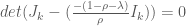
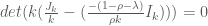
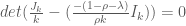
Now this is merely the equation for determining the eigenvalues of . Since, is idempotent the eigenvalues of must be either zero or one. In fact, since this matrix has rank one, has eigenvalues one with multiplicity one and zero with multiplicity . Therefore the eigenvalues of can be found by setting and . This yields with multiplicity and with multiplicity which are exactly the eigenvalues of .

Cheers.

A good excerpt from this article, By Gary Kreps, Ph.D, and Rebecca Goldin, Ph.D, November 17, 2009:

“Unlike the seasonal flu, H1N1 frequently attacks children. The CDC calculates that 179 flu-related pediatric deaths have occurred in the U.S since last April. Of these, one was due to the seasonal flu and 156 were due to H1N1. (The other 22 were due to a Type A influenza with an unidentified sub-type.) Compare those figures to the 2006-2007 flu season, when only 68 total pediatric deaths were linked to the seasonal flu. Thus, H1N1 has killed almost twice as many kids in the first month of this year’s flu season as the seasonal flu killed in an entire year during 2006-2007. The stakes are high for pregnant women as well, who constitute about one percent of the population but six percent of the deaths attributed to H1N1.

The media could help parents sort this out by framing this story in terms of comparative risk. Some parents may be willing throw the dice, reasoning that the absolute risk to their children is low. Instead they should compare the risk with that of other viruses for which vaccinations are now standard. Chicken pox, which used to take kids out of school for one or two weeks, was widespread until a vaccine became available in 1995. Before the vaccine, 100 to 150 people died each year from the disease, and more than 10,000 were hospitalized. This cost to society was considered high enough that 46 states now require children to get vaccinated in order to attend school.

As this comparison makes clear, the decision to vaccinate against H1N1 should be a slam dunk. The danger may not be apocalyptic, but it is very real. Unless America’s parents get this message, it is their children who will suffer most from confusion and misinformation. In fact, once you get past the conspiracy theories and myths, the development of the H1N1 vaccine is a genuine success story of government and industry working together to serve the public interest. But it’s being undermined by a failure to get the real story out to the very people whose lives may depend upon it.”

Cheers.

Let me start by saying I’m not an expert on global warming. I’m absolutely sure the earth is getting warmer (think melting ice caps) and very sure that it is caused by humans (green house gases). But who knows. Remember, if someone yells their dissenting opinion loud enough, it becomes fact, right?

Anyway, I’ve read some articles about how global warming has “stopped” in the last ten years. For instance, this article: “Climatologists Baffled by Global Warming Time-Out” states: “At present, however, the warming is taking a break,” confirms meteorologist Mojib Latif of the Leibniz Institute of Marine Sciences in the northern German city of Kiel. Latif, one of Germany’s best-known climatologists, says that the temperature curve has reached a plateau. “There can be no argument about that,” he says. “We have to face that fact.”

It goes on to say: “Even though the temperature standstill probably has no effect on the long-term warming trend, it does raise doubts about the predictive value of climate models, and it is also a political issue. For months, climate change skeptics have been gloating over the findings on their Internet forums. This has prompted many a climatologist to treat the temperature data in public with a sense of shame, thereby damaging their own credibility.”

This sounds like he is claiming that the warming has stopped. I disagree with this. You can have a system that is, on the average increasing over the long term, while still observing very flat or even declining trends when we know the overall system is increasing. That doesn’t mean that the system isn’t increasing, it just means we’ve seen one realization of the random system that hasn’t increased entirely by chance.

Here is a simulation experiment. (All these numbers are made up, but they prove the point):
Consider at year 1 the average temperature is 75 degrees. Call this x[1]. Then at year two we observe a realization from a normal random variable whose mean is 1.005*75 with standard deviation 1. Call this x[2]. x[3], the temperature in the the third year, will than be an observation from a normal random variable with mean 1.005*x[2] and standard deviation 1.

Over the long run this is an increasing sequence, but let’s look at what happens in the relatively short term. I simulated 10,000 of these such chains for 100 “years” each.

After 5 years 20.4% of these sequences we below the starting temperature of 75 degrees. After 10 years, 12.8% were below 75 degrees. Think about that. We have a known increasing sequence and after 10 years, 12.8% of them ended below where they started. Global warming is like this. We can see small periods of decline, in fact we EXPECT to see small periods of decline, within this increasing sequence.

What happens when we look at this sequence after 50 years? 0.006% are below the starting temperature of 75 degrees. After 100 years, 0 are below 75 degrees.

So to say that global warming is “taking a break” based on ten years of evidence seems like bad science to me. And this is certainly not evidence invalidating the long term usefulness of climate change models.

Cheers.