From flight stats, describing a flight that is the first leg of a two-leg itinerary I’m flying in the near future – obviously this is the sort of flight where one is interested in knowing whether it tends to be on time, because one does not like being stuck in Charlotte:
This flight has an on-time performance of 84%. Statistically, when controlling for sample size, standard deviation, and mean, this flight is on-time more often than 95% of other flights.
I didn’t realize one could control for standard deviation and mean.
(Presumably controlling for “sample size” could mean some Bayesian approach, where if there is a small amount of data for a flight they tend to give moderate predictions. This is probably not too influential as flight stats uses a sixty-day window.)
NCAA Basketball Rankings – 2/26/2013
Updated 2-26-2013 at 12:19am
Resume ranks the teams based on what they have actually accomplished this season. Predictor ranks teams based on how well they are expected to perform in the future. Seed give the projected tournament seed for a team.
|
STATISTICS DECLARES WAR ON MACHINE LEARNING!
Well I hope the dramatic title caught your attention. Now I can get to the real topic of the post, which is: finite sample bounds versus asymptotic approximations.
In my last post I discussed Normal limiting approximations. One commenter, Csaba Szepesvari, wrote the following interesting comment:
What still surprises me about statistics or the way statisticians do their business is the following: The Berry-Esseen theorem says that a confidence interval chosen based on the CLT is possibly shorter by a good amount of $latex {c/\sqrt{n}}&fg=000000$. Despite this, statisticians keep telling me that they prefer their “shorter” CLT-based confidence intervals to ones derived by using finite-sample tail inequalities that we, “machine learning people prefer” (lies vs. honesty?). I could never understood the logic behind this reasoning and I am wondering if I am missing something. One possible answer is that the Berry-Esseen result could be…
View original post 556 more words
March Madness Preview
Using data from the 2012-2013 NCAA basketball season, I’ve ranked all of the division 1 teams in two ways. First, I have build a retrospective model for the season ranking all of the teams based on what they have actually accomplished so far this season. These rankings give weight to individuals games based on margin of victory and weight strength of schedule a little bit more heavily than most models. I used these rankings to create a tournament bracket by taking the highest rated team from each conference plus the next 37 highest rated teams as at large bids. Once this bracket was created, I used my prospective rankings to predict the games. The results are here.
I’m sure everyone out there will let me know what I got wrong.
Cheers.
NCAA Basketball Rankings – 2/9/2013
Updated 2-9-2013 at 12:07am
|
NCAA Basketball
|
NCAA Basketball Rankings – 2/3/2012
Updated 2/3/2013 at 12:34pm
Indiana reclaims the top rankings after defeating Michigan last night, while previous number 2 Kansas falls three spots to number 5 after a loss to Oklahoma State.
Oregon, Wichita State, and Colorado State all fell out of the top 25. Oregon and Wichita State are both on tow game losing streaks.
Oklahoma State jumps into the top 25 after beating Kansas (at Kansas!) along with UNLV and New Mexico.
|
What time does the Superbowl start? (and predictions)
6:30.
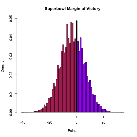
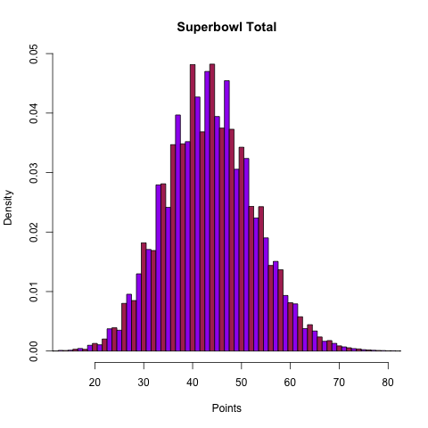
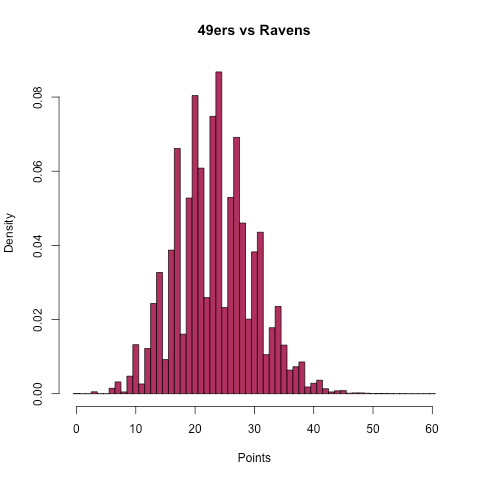
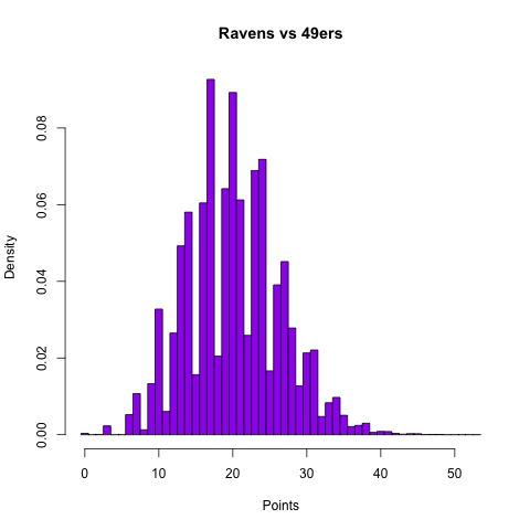
I’ve previously released my Super Bowl pick here, but I’ve also decided to release my forecast for the box score of the game and some visualizations of the distributions of team scoring, totals, and margin of victory as a preview for what I’m going to try to do in the 2013 season.
So, here is my predicted box score of the game:
| Team | Score | First Downs | Rushing Yards | Passing Yards | Total Yards | Turnovers |
| 49ers | 23.3 | 19.5 | 149.2 | 201.8 | 351.0 | 1.48 |
| Ravens | 20.2 | 18.4 | 108.1 | 223.3 | 331.4 | 1.59 |
Some selected probabilities:
| Team | Win | Cover (4.5) | Cover (3.5) | Win 10 or more | Overtime | Over/Under (47) |
| 49ers | 63.2% | 43.5% | 48.3% | 24.5% | 4.9% | O 29.5% |
| Ravens | 36.8% | 56.5% | 51.7% | 8.5% | 4.9% | U 66.2% |
Cheers.
I didn’t know this either!
I have been working with R for some time now, but once in a while, basic functions catch my eye that I was not aware of…
For some project I wanted to transform a correlation matrix into a covariance matrix. Now, since cor2cov does not exist, I thought about “reversing” the cov2cor function (stats:::cov2cor).
Inside the code of this function, a specific line jumped into my retina:
What’s this [ ]?
Well, it stands for every element $latex E_{ij}$ of matrix $latex E$. Consider this:
> mat
     [,1] [,2] [,3] [,4] [,5]
[1,]   NA   NA   NA   NA   NA
[2,]   NA   NA   NA   NA   NA
[3,]   NA   NA   NA   NA   NA
[4,]   NA   NA   NA   NA   NA
[5,]   NA   NA   NA   NA   NA
With the empty bracket, we can now substitute ALL values by a new value:
> mat [,1] [,2] [,3] [,4] [,5] [1,] 1 1 1 1…
View original post 55 more words
Hilary: the most poisoned baby name in US history
I’ve always had a special fondness for my name, which — according to Ryan Gosling in “Lars and the Real Girl” — is a scientific fact for most people (Ryan Gosling constitutes scientific proof in my book). Plus, the root word for Hilary is the Latin word “hilarius” meaning cheerful and merry, which is the same root word for “hilarious” and “exhilarating.” It’s a great name.
Several years ago I came across this blog post, which provides a cursory analysis for why “Hillary” is the most poisoned name of all time. The author is careful not to comment on the details of why “Hillary” may have been poisoned right around 1992, but I’ll go ahead and make the bold causal conclusion that it’s because that was the year that Bill Clinton was elected, and thus the year Hillary Clinton entered the public sphere and was generally reviled for not wanting to…
View original post 1,430 more words
