This past Thursday, I attended a book reading at Booklinks Booksellers in Northampton, MA. Benjamin Baumer and Andrew Zimbalist were reading from their new book, The Sabermetric Revolution: Assessing the Growth of Analytics in Baseball. Approximately 30 baseball starved fans braved the cold New England night to learn a few things about sabermetrics and baseball analytics. It was a very informative hour that included the reading of a few book excerpts, a lively Q&A session, and complimentary wine. What could be better on a February night than good baseball discussion and free alcohol!

Andrew Zimbalist is the Robert A. Woods Professor of Economics at Smith College and a noted sports economist who has written numerous books concentrating on the business of sports, especially baseball. Benjamin Baumer is a Visiting Assistant Professor at Smith College who spent eight years working as a Statistical Analyst for the New York Mets. The Sabermetric Revolution is their first joint project.

Professor Zimbalist opened up the event by reading from the preface of their new book. At the outset, Zimbalist made clear that a major focus of the book is debunking numerous statistical myths and cause and effect relationships about baseball that were promulgated in the book Moneyball by Michael Lewis and the subsequent movie starring Brad Pitt. The authors take no punches in lambasting Lewis for gross inaccuracies in his 2003 book. Zimbalist stated that Michael Lewis fell in love with a story and dramatically overplayed some of the success of the 2002 Oakland Athletics as sabermetric in source.

Professor Baumer continued the event by reading a brief excerpt from Chapter 2. He discussed the rise in use by most MLB franchises of sabermetric analysis in direct response to the popularity of Moneyball.  Considering Baumer’s direct experience with the industry, his insight into the actual operations and use of statistics in baseball was fascinating and very eye opening.

After a joint discussion between the two authors about the use and application of the various baseball analytical metrics currently en vogue, the floor was opened to questions from those in attendance.  Many of the audience questions focused on Baumer’s experience with the Mets and his opinion of the utility of sabermetrics on the baseball industry. The authors made a point of stating that many newly coined statistics are still in their infancy and their exact utility has yet to be truly discovered. They specifically mentioned Ultimate Zone Rating (UZR) as a statistic that has yet to prove its true usefulness as a real world baseball application.

One audience member asked if players have used these advanced metrics to change their approach to the game. Baumer responded that when he was with the Mets, the baseball operations staff pleaded with the field manager and coaches to convince Jose Reyes to walk more from the leadoff spot. He did, and his impact on the field from the top of the batting order substantially increased. However, Baumer noted that this was an exception to the general rule. In a broader sense, using sabermetrics to find the player you need rather than to change the player you have seems to be the more successful application.

One gentleman asked if there has been any evidence that other sports use statistical analysis. The authors responded that while baseball is unique in that players have such individualized contributions to their team, there has been some proof of its applicability to football and basketball in particular.  Baumer noted that current Boston Celtics coach Brad Stevens used statistical analysis in his time coaching the overachieving Butler University Bulldogs.

The evening closed with Zimbalist and Baumer reemphasizing the purpose of their book. Ten plus years after Moneyball was published, they wanted to take a critical look at what parts of sabermetrics work, what parts don’t, and how the sports and industry of baseball is evolving while using analytical tools.

As an aside, I am currently reading the book and thus far I’m most fascinated by the career trajectories of the much heralded 2002 Oakland Athletics amateur draft class. Lewis went out of his way to talk about the advanced statistical tools used to make the draft selections, and now 11 years later Baumer and Zimbalist revisit the draft and the players that the Athletics took. Needless to say, the actual careers of most of the players highlighted by Lewis did not exactly match the accolades espoused in the book.

If you are interested in baseball and sports analytics, this book is a must read.

I just came across this article with the following headline:

As many as 988 million birds die annually in window collisions.

Wait, what?  Almost a BILLION (with a “B”) birds are killed every year by flying into windows?  That’s an outrage!  Let’s tear down all of our building and get rid of all our windows in defense of our feathers friends!

No wait.  Actually, let’s take a step back and see what’s happening here.  First, where does the 988 million number come from?  It comes from this study: Bird–building collisions in the United States: Estimates of annual mortality and species vulnerability in some journal called “The Condor”.  And actually what they say in their abstract is:

Based on 23 studies, we estimate that between 365 and 988 million birds (median = 599 million) are killed annually by building collisions in the U.S.

So 988 million (nearly a BILLION!) is the upper threshhold of their interval estimate of annual bird deaths by window collisions.    But why did the Washington Post leave out the interval estimate and only mention the upper bound?  I’d guess because it’s a more sensational headline.  (If I’m wrong, please let me know what the reason is.)  C0me on media, you’re better than this.

So just to be clear, what the studied actually “showed” is that they estimate that somewhere between 365 and 988 million birds with a median of 599 million are killed in window collisions annually.  Even if their methods are completely sound their median estimate is about 40% lower that the sensational upper limit.  (Which I suppose would translate into 40% fewer clicks.)  So even if they are correct, I feel like the media is being sensationalist about their “findings”.

BUT!  BUT! I suspect strongly that their methods are not only not completely sound, I suspect their methods are barely acceptable.  In fact, I’ve actually reviewed the statistical methods employed by this same exact author, Dr. Scott R. Loss, before for a similar study that claimed that cats were killing incredibly large numbers of birds.  My complete report can be viewed here.  (Full disclosure: I was a paid consultant for Alley Cat Allies when I wrote that; They are not paying me for this blog post.)  So, Dr. Loss doesn’t have the best statistical track record in my opinion, though he may be a fine ornithologist (he was, after all, the Outstanding Conservation Biology Student of 2009-10.  Congrats!).  In my professional opinion, as I have stated before, the methods employed in the article “The impact of free-ranging domestic cats on wildlife of the United States” have almost no statistical validity.

While I haven’t fully reviewed the methods in the new paper about bird collisions, I suspect that the same or very similar methods have been employed to reach these astronomically sensational numbers.  Again, as I have said before, these numbers may be completely correct (though I suspect they are not), but the statistical methods used to arrive at these numbers are extremely shoddy.

And guess what?!?! Dr. Loss looks like he has a whole series of these papers coming out!  Check out his CV under submitted papers.  Vehicle collisions, power lines, wind farms!

So Dr. Loss if you’re reading this, please PLEASE consult with a statistician.  Also, if you’d like to respond to my criticism, I’d be happy to post your unedited response on my blog.

Cheers.

P.S.  By the way, one BILLION (that’s 1,000,000,000) birds per year would mean that almost 32 birds PER SECOND were dying on average in every second, day and night, of every day all year round JUST IN THE UNITED STATES!

His decision to punt from the Seattle 39-yard line with his team trailing 29-0 early in the third quarter elevated football-coach risk aversion to something more like hyper-milquetoast performance art. 

-Josh Levin

Full article

Introduction

Recently I tweeted the following question: “Does the spread of an NFL game predict how exciting the game will be?”  If closer games are considered more exciting (I think most people will agree with this), then games with smaller spreads should be, on average, more exciting than games with larger spreads.

So how do we test this?  The first big question that we need to answer is this: how do we quantify “excitement” of a game?  Luckily, someone has already done this for us. Advance NFL Stats calculates a statistics they call the “excitement index” (EI).  It is defined as follows on their website:

Excitement Index (EI) – The measure of how exciting a game is. EI measures the total movement of the Win Probability (WP) line during a game. The more that WP fluctuates, the more dramatic, uncertain, and exciting a game is.

I think this is a great definition of excitement, and whether or not you totally agree that this is or is not the best way to measure this, it is certainly a great place to start.

So to begin with I collected the EIs and spreads for all regular season games from 2010 through 2013 for a total of 1024 games.

Summaries of the data

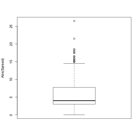
Looking at a summary of the absolute value of the spread over these 1024 games we find that the average spread is 5.44 points with a median of 4.  The inner quartile range of spreads in from 3 to 7.625 and the minimum spread over this time was 0 with a maximum of 26.5(!).

The average EI is 4.036 with a median of 3.9.  The inner quartile range of the EI is from 2.7 through 5.2.  The least exciting game over this time period was measured to be 1.1 with the most exciting game at 9.8.

Regression Model

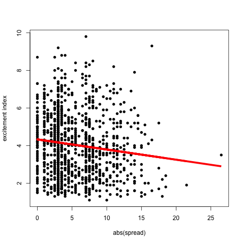
Next, I fit a simple linear regression model with excitement as the response variable and absolute value of the spread as the predictor.  The fitted regression parameters are:

• Intercept: 4.33023 (p-value < 2e-16)
• Spread: -0.52 (p-value 4.58e-05)

This means that for ever two point increase in spread, we lose, on average, about 1 point of excitement index.  In other words with a spread of 0, the average predicted excitement index (EI) of a game is 4.33023.  This is about the 60th percentile of all EIs from 2010-2013.  A spread of 3 yields a predicted excitement index of 4.168 with is about the 55th percentile of all excitement indices.  When the spread jumps to 7 points, the average excitement level is about 3.95 which is about the 51st percentile of EI.

What can we expect about the most exciting game in a playoff weekend?  If we have four games all with spreads of 0, we can expect that the most exciting game will be about a 6 EI, which is about the 85th percentile of EI.  If all four games have a spread of 3 points we can expect the most exciting game to be about 5.9 EI, which is about the 84th percentile of EI, and if all 4 games have spreads of 7 we expect the most exciting game to be about 5.67 which is around the 81st percentile of games.  So what’s the difference between a 5.7 and a 6 for instance?  Here is an example of a 6 and here’s an example of a 5.7.  I guess the answer is not much.

What can we expect in the Super Bowl?

The Super Bowl spread tonight is 2.5 points with Denver favored.  This gives us an expected excitement index of 4.19523, which is about the 55-th percentile of exciting games.  So we should expect the game tonight to be more exciting that than more than half of all regular season games played in the last four years.  And that is exciting.

Cheers.

Some interesting stupid facts:

• In years when Punxatawny Phil predicts early spring the average Super Bowl total is 51.67 whereas when long winter is predicted the average total is 44.03. I assume this is because it’s easier to score points in warm weather.
• The NFC team averages 30.42 points when Phil predicts early spring as opposed to an average of 23.23 points for a prediction of long winter.  This means that the NFC team gains about 1 extra touchdown for a prediction of early spring.
• The average margin of victory with a prediction of early spring is 18.5; When long winter is predicted the average margin of victory is 12.6.

Update: Phil emerged this morning at 7:28am and predicted 6 more weeks of winter.  This means we can expect a low scoring, close game with no advantage for the NFC.  This is reflected in the current Super Bowl line of Denver -2.5

Cheers.

Denver Broncos vs Seattle Seahawks

Prediction: Seahawks 26-24

Win Probability: Seahawks 54.72%

SU: Seahawks +2.5

Pick: Seahawks +115

OU: Over 46.5

6:30 pm.  On FOX.

Cheers.