JSM (in the wild)
I’ve been in Vancouver the past week for the Joint Statistical Meetings (JSM) . Here is a collection of my thoughts and comments from the few days I was at the conference.

On Monday I went to the section on Survey Research Methods and saw Meena Khare, of the National Center for Health Statistics (NCHS) and Laura Zayatz of the United States Census give talks. They both spoke about measures that their institutions go through to release data to the public. The NCHS looks for uncommon combinations of variables that could be used to possible de-identify the data. Both organizations first remove obvious identifiers and then go on to make the released data more private. For instance, if the number of observations with a unique combination of variables in a data set is n and the number of observations with the unique combination is N, they would consider any combination of variables where n/N<.33 at risk for disclosure. At the U.S. Census, they have used something called data swapping to protect public release data sets in the last two Censuses (2000 and 2010). Along with data swapping, the Census will also be using partially synthetic data to maintain confidentiality to protect individual privacy in public release data in 2010.
Several things strike me about this.
-The methods that these organizations use to protect confidentiality are certainly going to increase privacy compared to a release of raw data, however, there doesn’t seem to be any way to know that what is being done is providing “enough” privacy.
-It’s clear that many different government organizations have issues which require some use of disclosure limiting techniques, however, it seems that each organization is creating its own rules and there is limited discussion going on between organizations to conceive of a standard policy for data sharing.
-There doesn’t actually seem to be any definition of what is considered a disclosure. For instance, if government data is released and I discover through some technique that someone definitely has HIV, then clearly a disclosure has taken place. However, if I use the same data to discover that someone definitely does not have HIV, a disclosure has still taken place, but the consequence is much less damaging. Furthermore, consider a situation where prior the the data release, I know a particular individual has a 50 percent chance of having HIV. After the data release, I can infer that there is a 99 percent chance that they have HIV. Clearly, I would consider this a disclosure. But what if the probabilities shift from only 50 percent (pre-data release) to 75 percent (post-data release) or 50 percent to 55 percent. At what point is “too much” information being released. It seems as if this issue receives less attention than is warranted.
-Finally, I believe that the ultimate solution to the disclosure problem is a careful combination of policy and disclosure limiting techniques. Policy issues include defining how much privacy must be maintained by a given technique, as well as, legal consequences for knowingly disclosing private information. Statistics has an obligation to provide increasingly improving statistical disclosure techniques along with metrics for measuring the privacy of a given technique.
Later on Monday, I saw the tail end of the talk by David Purdy titled “Statisticians: 3, Computer Scientists: 35”. The abstract for the talk was:
“John Tukey and Leo Breiman warned us that a day would come when statistics would need to focus more on computing, or risk losing good students to computer science. The Netflix Prize provides many examples of how our field needs to do more.
In the top 2 teams, participants with a computer science background vastly outnumbered those with a statistics background. There are a number of lessons that the field of statistics can learn from the fact that undergraduates in CS were well equipped to compete, while statisticians at all levels were not well prepared to implement advanced algorithms.
In this talk, I will address methodological issues arising with such a large, sparse dataset, how it demands serious computational talents, and where there is ample room for statistics to make contributions.”
I only saw the end of the talk, but I feel like I got the point. He notes how programs in statistics need to expose students to more aspects of computing. One quote from his talk that particularly shocked me was from a prominent statistician referring to the Netflix prize data set: (I’m paraphrasing) “I can’t do anything with the data, there is just too much of it.” (If anyone knows the actual quote, I would love to have it). Too little data may often be a problem, but too much data should be a blessing, rather than a curse.
When he is talking about computing he is referring to implementing complex algorithms to analyze the data, however, in my experience I have seen people struggle with simply managing data of this size. This is a simple problem to deal with, but, in my experience, I have both had this happen to myself and seen it happen to others. When I was in grad school working towards my master’s degree right out of undergraduate, we were given a problem in a consulting class with a “large” (several thousand observations) amount of data (well, “large” to someone with no experience managing data.) We (my group) knew exactly what we wanted to do with the data, but we are unable to manage the data in a way that would make it useful for analysis. So we did nothing. The moral of the story here is that, while we were taught well the techniques which were useful for analyzing the data, we were never taught and had never learned any useful data manipulation techniques, rendering our statistical educations useless. It was not until I got my first job that I learned, out of necessity, data management techniques including SAS data steps, SAS macros, and SQL.
When I returned to school to pursue a Ph. D., I saw many students with no work experience struggling through all of the same problems that I had with managing data. The same old “I know exactly what I want to do, but I can’t organize the data.” Often times in grad classes, books or teachers will describe a data set as “large” when it has several hundred or several thousand observations. This seems inadequate preparation for working in industry, as my first jobs often dealt with data sets with millions of observations and, later, a summer consulting project involved billions of observations.
Currently, there are no required computing or data management classes in my program for earning a Ph. D. in statistics. I think there should be a required class in every statistics program covering data management issues and, at least, a solid introduction to programming.
After, David Purdy’s talk, Chris Volinksy (Follow on Twitter) and he took questions. One interesting question that came up was about a second Netflix prize. However, Chris noted that this had to be cancelled because of privacy concerns. I’ve written before (or at least posted on Twitter) about some researchers who claim to have de-anonymized the data from the Netflix prize and, as a result, a lawsuit has been filed. (Netflix’s Impending (But Still Avoidable) Multi-Million Dollar Privacy Blunder) Whether you agree with canceling the prize over privacy concerns or not, it is clear that disclosure limitation is currently a big issue that certainly cannot be ignored.
On Tuesday, I went to one of the sports research sections and saw two talks before I left to go see a talk about partially synthetic data in longitudinal data. The first speaker, Shane Jensen, spoke about evaluating fielders abilities in baseball using a method he proposed called Spatial Aggregate Fielding Evaluation (SAFE). The previous link explains how their evaluation of players works and gives measures of performance for each player. Probably, the most shocking result of his work is that, averaged over 2002-2008, SAFE evaluated Derek Jeter as the worst shortstop who met the minimum number of balls in play (BIP). Alternatively, SAFE rates Alex Rodriguez as the second best shortstop over this same period, even though he now plays third to allow Jeter to play SS.
The next speaker was Ben Baumer, statistical analyst for the Mets (and native of the 413 area code). He spoke about his paper, “Using Simulation to Estimate the Impact of Baserunning Ability in Baseball“. One of the interesting things I took away from his talk is that he claims that players’ speed used to break up a double play is one of the important aspects of base running, but this is often largely or completely ignored as an evaluation tool of a players base running ability.
Before I end, I’d like to say thanks to all the speakers that I saw speak this past week and, finally, I’ll leave you with a view of Vancouver from the convention center.
Cheers.

Twitter and Emoticons (in the wild)
According to infochimps.org these are the 25 most used emoticons on twitter.com. Download the whole data set yourself here.
1 13458831 🙂
2 3990560 :d
3 3182129 😦
4 2935301 😉
5 2082486 🙂
6 1461383 =)
7 1439234 :p
8 1013758 😉
9 979947 (:
10 669086 xd
11 656784 ![]()
12 595140 =d
13 527391 =]
14 490897 :]
15 398246 😦
16 367208 😮
17 350291 d:
18 332427 ;d
19 321328 =(
20 310343 =/
21 252914 =p
22 247794 ):
23 240355 :-d
24 217052 😐
25 179184 ^_^
Info about the data:
“This data comes from a scrape of the Twitter social network conducted by the Monkeywrench Consultancy. The full scrape consists of 35 million users, 500 million tweets, and 1 billion relationships between users.
This dataset is a corpus of tokens collected from tweets sent between March 2006 and November 2009. A “token” is either a hashtag (#data), a URL, or an emoticon (smiley face — ;)). Think about comparing this data to the stock market, new movies, new video games, or even trendingtopics.org. For example, use it to look at the social networking adoption of Google Wave on the rate of its mentions.”
Actually, all that I got in the free download was emoticon counts for the period between March 2006 and November 2009. So I got to thinking about what you could possibly do with this data in a useful way. What I was thinking about doing is trying to get a break out of emoticon usage by day or hour over the last few years. Then try to look for spikes in smileys, or frowns, or winks and see if these spikes are related to anything. Do you think we can measure world happiness or sadness based on emoticon use? (Probably not, but it’s an interesting thought, right?)
Cheers.
JSM (in the wild)
The Joint Statistical Meetings (JSM) are coming up in the first week of August in Vancouver. StatsInTheWild will be in attendance.
Here are the StatsInTheWild suggestions for interesting talks to attend.
Disclosure Limitation and Confidentiality:
A New Approach to Protect Confidentiality for Census Microdata with Missing Values Yajuan Si, Duke University; Jerome P. Reiter, Duke University. Monday, August 2, 2010 10:35 AM
Disclosure Avoidance for Census 2010 and American Community Survey Five-Year Tabular Data Products
Laura Zayatz, U.S. Census Bureau; Paul Massell , U.S. Census Bureau; Jason Lucero, U.S. Census Bureau; Asoka Ramanayake, U.S. Census Bureau. Monday, August 2, 2010 11:15 AM
Multiple Imputation Method for Disclosure Limitation in Longitudinal Data
Di An, Merck & Co., Inc.; Roderick Joseph Little, University of Michigan; James W. McNally, University of Michigan
11:35 AM
Balancing Individual Privacy with Access to Data for Policymaking
Panelists:
Stephen E. Fienberg , Carnegie Mellon University
Nancy M. Gordon, U.S. Census Bureau
Michael Lee Cohen, Committee on National Statistics
Tom Krenzke, Westat
Ed J. Christopher, Federal Highway Administration
Stephen Gunnells, The Planning Center
Wednesday, August 4, 2010 : 2:00 PM to 3:50 PM
Sports:
Spatial Modeling of Fielding in Major League Baseball Shane Jensen, The Wharton School, University of Pennsylvania. Tuesday, August 3, 2010 10:35 AM
Exploring the Count in Baseball Jim Albert, Bowling Green State University. Tuesday, August 3, 2010 11:35 AM
False Starts and Alternative Hypotheses Michael Rotkowitz, The University of Melbourne
Multiple Imputation:
Multiple Imputations for Survey Sampling and Their Diagnostics – Invited – Papers. Sun, 8/1/10, 2:00 PM – 3:50 PM
This entire section is worth attending.
Law:
Formal Statistical Analysis Provides Sounder Inferences Than the U.S. Government’s ‘Four-Fifths Rule’: Examining the Data from Ricci v. DeStefano. Weiwen Miao, Haverford College; Joseph L. Gastwirth, Washington University. Wednesday, August 4, 2010 11:15 AM.
See you in Vancouver.
Cheers.
Social Networks (in the wild)
I attended the New England Statistics Symposium (NESS) last Saturday, and I’ve been meaning to write about one of talks I saw. After lunch, I went to the Columbia section so I could see the talk about multiple imputation using chain equations. The MI talk was the second in the section, so I sat through the first talk presented by Tian Zheng (Tian’s Blog) which turned out to be very interesting. The talk was about using social networks to learn about at risk populations.
My understanding of this is that a survey could be given asking people questions about who they know rather than about themselves. For instance, instead of asking “Is your name Michael?” and “Are you homeless?” ask “How many Michaels do you know?” or “How many homeless people do you know?” Then using the responses to these questions, researchers can estimate how large at risk populations are. And they can do this without ever asking people who are in the at risk population! Really neat.
Why is this useful?
This excerpt from this flyer that was created to describe the method to a general audience says it very well:
“AT-RISK POPULATIONS: At-risk populations can be hard to access (eg. homeless) or reluctant to admit their status for fear of others finding out (eg. HIV/AIDS, drug abusers, sex workers). Statisticians learn about these populations through their friends and acquaintances. Instead of asking if a person uses IV drugs, ask ‘How many IV drug users do you know?’ and use social structure to learn about the person using IV drugs.”
Really, really neat stuff.
Cheers.
NCAA Basketball top 25: March 23,2010 (in the wild)
StatsInTheWild NCAA Basketball top 25:
(Boldindicates team is still in the NCAA tournament, italics indicate change from last week)
1. Kansas 0
2. Kentucky 0
3. Syracuse 0
4. West Virginia 0
5. Duke +2
6. Cornell NR
7. Kansas State +2
8. Purdue +5
9. New Mexico -3
10. Northern Iowa +13
11. Butler +6
12. Baylor -1
13. Temple -5
14. Tennessee +1
15. Texas A&M -1
16. Ohio State +3
17. Villanova -12
18. Xavier +6
19. Georgetown -9
20. Pittsburgh -8
21. Michigan State NR
22. Missouri NR
23. Gonzaga NR
24. Maryland -3
25. San Diego State NR
Other Notables: Saint Mary’s (26), Washington (33)
Cheers.
NCAA Basketball Sweet Sixteen edition (in the wild)
Well there are 16 teams left and my bracket is in shambles.
Let’s review the predictions from last week.
My failures:
Two of my final four teams are gone (Villanova and Kansas) including my champion (Kansas) so I won’t win any office pools this year.
My triumphs:
-A lot of my predictions from my tournament preview came through including both of my predicted lower seed first round locks (Northern Iowa and Missouri).
-I had Northern Iowa in my top 25 . Certainly not higher than Kansas, but definitely a top 25 team.
-My model ranked Cornell 18th and I ignored it figuring it was a fluky part of the model. (Similar to how I have Oral Roberts ranked 8th and Sam Houston State ranked 2nd using the raw data.) I guess Cornell really is that good. This win over Wisconsin should shoot them up in my rankings when they come out tomorrow.
Some observations:
-Washington is really bad. They beat a mediocre Marquette team and then a New Mexico team that lost to San Diego State in its conference tournament. West Virginia is going to massacre Washington. (Note: Marquette lost 51-50 to DePaul this season. DePaul was 1-17 in the Big East. Yikes.)
-The Kentucky-Cornell game is going to be really interesting. Kentucky is loaded with super talented Freshman who are thinking about the NBA and millions of dollars and Cornell is stacked with seniors who are thinking about grad school next fall.
My picks:
-Kentucky over Cornell: Cornell keeps it close in the first half, but Kentucky’s superior talent takes over. They win by 10.
-West Virginia over Washington: West Virginia is going to kill them. I see them winning by 15-20 points.
-Duke over Purdue: This is an interesting match-up. Purdue had thoughts of a number 1 seed going into their conference tournament and they ended up with a 4. I’ll be interested to see how they play in this one.
-Baylor over Saint Mary’s: Baylor has beaten a 14 and an 11 seed. Saint Mary’s is a 10. I’m not sure what that means, but the total of the seed of Baylor’s first three opponents is 35. That has to be the highest total of a first three opponents, right? Anyway, this one will be close. Baylor by 3.
-Northern Iowa over Michigan State: I had Northern Iowa in top 25 at the beginning of the tournament and they are still there. I had Michigan State out of my top 25. Northern Iowa by 7. (Michigan State has made the Sweet Sixteen three years in a row.)
-Tennessee over Ohio State: How many games does Ohio State have to win in a row to convince me they are for real? 1 more. But I doubt it. Tennessee by 10.
-Syracuse over Butler: Syracuse by 5…..unless Shelvin Mack hits a million threes again. Then who knows.
-Kansas State over Xavier: Kansas State looks good. really good. (Note: Xavier has made the Sweet Sixteen three years in a row.)
Final Four picks:
Kentucky, Duke, Syracuse, and……(wait for it)…………Northern Iowa. Northern Iowa beat Kansas, surely they can beat Michigan State, and Ohio State or Tennessee, right?
Finals:
Syracuse vs Kentucky
Champion:
Kentucky 72-68
Can’t wait until next Monday when I get to see just how wrong I am again.
Cheers.
NCAA Basketball top 25 (in the wild)
(Bold Indicates Sweet Sixteen team.)
StatsInTheWild top 25:
1. Kansas
2. Kentucky
3. Syracuse
4. West Virginia
5. Villanova
6. New Mexico
7. Duke
8. Temple
9. Kansas State
10. Georgetown
11. Baylor
12. Pittsburgh
13. Purdue
14. Texas A&M
15. Tennessee
16. Texas
17. Butler
18. Vanderbilt
19. Ohio State
20. Marquette
21. Maryland
22. Richmond
23. Northern Iowa
24. Xavier
25. BYU
Inexplicable regular season losses:
Penn beat Cornell 79-64
Indiana beat Pittsburgh 74-64
Brown beat Princeton 57-54
Evansville beat Northern Iowa 55-54
Cheers.
NCAA Basketball (in the wild)
It’s that magical time of year again. The three weeks the rest of the country and I care about college basketball. Check out the StatsInTheWild NCAA basketball top 25.
So here it is. The StatsInTheWild annual NCAA tournament preview.
Teams that should have gotten in but didn’t:
Seton hall – I realize it’s hard to take a team that went 9-9 in their conference, but it’s the big east. it really is that good.
Virginia Tech – They should have been in easy. Although 2 losses to lowly Miami, including once in the ACC tournament is really bad.
Mississippi State – A good regular season and a very good run in the SEC tournament. Should have been in.
Teams that should not have gotten in:
Minnesota – They lost to Michigan twice in February and they lost to Indiana who was 4-12 in the conference. And they were only 9-9 in the conference. The big 10 is the most over rated conference in football and basketball.
UNLV – Third in the Moutain West gets in but third in the ACC doesn’t? This was a bad at large bid.
Wake Forest – They finished 6th in the ACC at 9-7 in conference. How did Virgina Tech not get in again?
Georgia Tech – They finished 7th in the ACC at 7-9 in conference. How did Virgina Tech not get in again?
Best 16 seed: Lehigh
Best 15 seed: UC-Santa Barbara
Best 14 seed: Sam Houston State
Worst 1 seed: Duke
Worst 2 seed: Ohio State
Worst 3 seed: Pittsburgh
Worst 4 seed: Wisconsin
Most likely first round upsets:
(14) Sam Houston State over (3) Baylor
(12) New Mexico State over (5) Michigan State
(13) Wofford over (4) Wisconsin
(11 )Old Dominion over (6) Notre Dame
Most likely long shot upset:
(15) UC-Santa Barbara over (2) Ohio State
Lower seed lock:
(10)Missouri over (7) Clemson
(9) Northern Iowa over (8) UNLV
Sweet Sixteen:
All the one’s, two’s, and three’s along with (4) Maryland, (4) Butler, (5) Texas A and M, and (5) Temple.
Elite 8:
All the number one seeds and all of the number 2 seeds except Ohio State. Georgetown gets in.
So that’s (1) Kentucky, (1) Duke, (1) Syracuse, (1) Kansas, (2) Kansas St, (2) Villanova, (2) West Virginia, and (3) Georgetown.
Final 4:
(1) Kansas, (1) Kentucky, (1) Syracuse, (2) Villanova
Finals:
(1) Kansas vs (1) Kentucky
Champion:
(1) Kansas over (1) Kentucky 68-66
LaTeX and WordPress (in the wild)
Apparently, you can use LaTeX in wordpress. Alright, he is a practice problem I was working on for my exam in two weeks.
Let 


We seek 


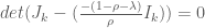
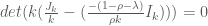
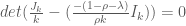
Now this is merely the equation for determining the eigenvalues of 


Cheers.
More H1N1 (in the wild)
A good excerpt from this article, By Gary Kreps, Ph.D, and Rebecca Goldin, Ph.D, November 17, 2009:
“Unlike the seasonal flu, H1N1 frequently attacks children. The CDC calculates that 179 flu-related pediatric deaths have occurred in the U.S since last April. Of these, one was due to the seasonal flu and 156 were due to H1N1. (The other 22 were due to a Type A influenza with an unidentified sub-type.) Compare those figures to the 2006-2007 flu season, when only 68 total pediatric deaths were linked to the seasonal flu. Thus, H1N1 has killed almost twice as many kids in the first month of this year’s flu season as the seasonal flu killed in an entire year during 2006-2007. The stakes are high for pregnant women as well, who constitute about one percent of the population but six percent of the deaths attributed to H1N1.
The media could help parents sort this out by framing this story in terms of comparative risk. Some parents may be willing throw the dice, reasoning that the absolute risk to their children is low. Instead they should compare the risk with that of other viruses for which vaccinations are now standard. Chicken pox, which used to take kids out of school for one or two weeks, was widespread until a vaccine became available in 1995. Before the vaccine, 100 to 150 people died each year from the disease, and more than 10,000 were hospitalized. This cost to society was considered high enough that 46 states now require children to get vaccinated in order to attend school.
As this comparison makes clear, the decision to vaccinate against H1N1 should be a slam dunk. The danger may not be apocalyptic, but it is very real. Unless America’s parents get this message, it is their children who will suffer most from confusion and misinformation. In fact, once you get past the conspiracy theories and myths, the development of the H1N1 vaccine is a genuine success story of government and industry working together to serve the public interest. But it’s being undermined by a failure to get the real story out to the very people whose lives may depend upon it.”
Cheers.
