Category Archives: R
One last post on field goals and presidential politics
I think I’ve finally finished these. Thanks to everyone for the good suggestions. These are based on this post yesterday.
Here are both Trump and Biden together. The first is Trump, the second Biden. It’s not quite symmetric, but it’s close. For instance, Biden winning Minnesota is about a 37 yard field goal. Trump winning Minnesota is a 57 yard field goal. It would be kind of cool if it worked in both directions, but it doesn’t quite work, unfortunately.
If you look at a bunch of states that Trump needs to win, like Florida, Michigan, Pennsylvania, Wisconsin, etc. they are all in the 60 (like Florida) to 70 (like Michigan) yard range. So for Trump to win he needs to him a few 60 yard field goals in a row (granted they are correlated, so it’s a little bit easier than that). But it’s not easy to hit a 60 yard field goal! But it does happen!


Cheers.

Biggest NFL Spread Changes in Rematches in 2018
The Bears just clinched the NFC North for the first time in, I want to say, 100 years, by beating the Green Bay Packers last weekend at Soldier Field. Their week 15 meeting was the second time these division rivals have played this season and their first meeting came way back in week 1 when Chicago blew a 20 point lead and they looked well on their way to a 5-11 season, while Aaron Rodgers looked like Superman. But that was a long time ago and everyone seems to have caught up to the idea that the Bears are good this year and Green Bay is not. And you can see this in the spreads for the two games.
In the first meeting at Lambeau Field in week 1, the Packers were 6.5 point favorites over the Bears, who covered despite losing in crushing fashion. 14 weeks later and spread for the Bears-Packers game at Soldier Field was Bears -5.5. That is a shift of 12 points.
Now some of this has to do with home field advantage. If two teams were essentially equal on a neutral field, you’d expect this difference to be about 6-ish (-3 at home and +3 away). But 12 seemed rather large to me, and I wondered if that was the largest shift in spreads in a rematch this year. While it is not, in fact, the largest, it is close. There were two matchups that had a larger shift in spreads. Stop reading and try to guess what those match-ups were.

Ok. You ready now? The largest difference this year was the Titans and Jaguars. In September the home Jaguars were favored by 10 over the Titans in week 3. In week 13, The Titans at home were favored by 5.5, for a 15.5 point swing. Coming in at number 2 was Atlanta and New Orleans. In their first meeting in week 3, the Falcons were favored by 2. In week 11, the Saints were favored by 12.5. The previously mentioned Bears and Packers came in at 3rd largest with a shift of 12.0.

The only other two double digit shifts were Buffalo-NY Jets and Dallas-Philadelphia. The Bill vs Jets shift happened in only 4 weeks. In week 10, the Jets were favored by 7, then in week 14 the Bills were favored by 4.5 . Rounding out the top five was the Cowboys and Eagles. In week 10, the Eagles were favored by 7 points then by week 14 the Cowboys were favored by 3.5. Here is the list of all of the shifts of at least 5:
- Jacksonville – Tennessee: 15.5
- Atlanta – New Orleans: 14.5
- Chicago – Green Bay: 12.0
- Buffalo – New York Jets: 11.5
- Dallas – Philadelphia: 10.5
- Kansas City – LA Chargers: 7
- Dallas – Washington: 6
- Miami – New York: 6
- San Francisco – Seattle: 5.5
- Baltimore – Cincinnati: 5.5
- Cleveland – Pittsburgh: 5.5
- LA Chargers – Oakland: 5.0
I’ll follow up on this when the season ends, and I also want to go back and look at past seasons.
Cheers.
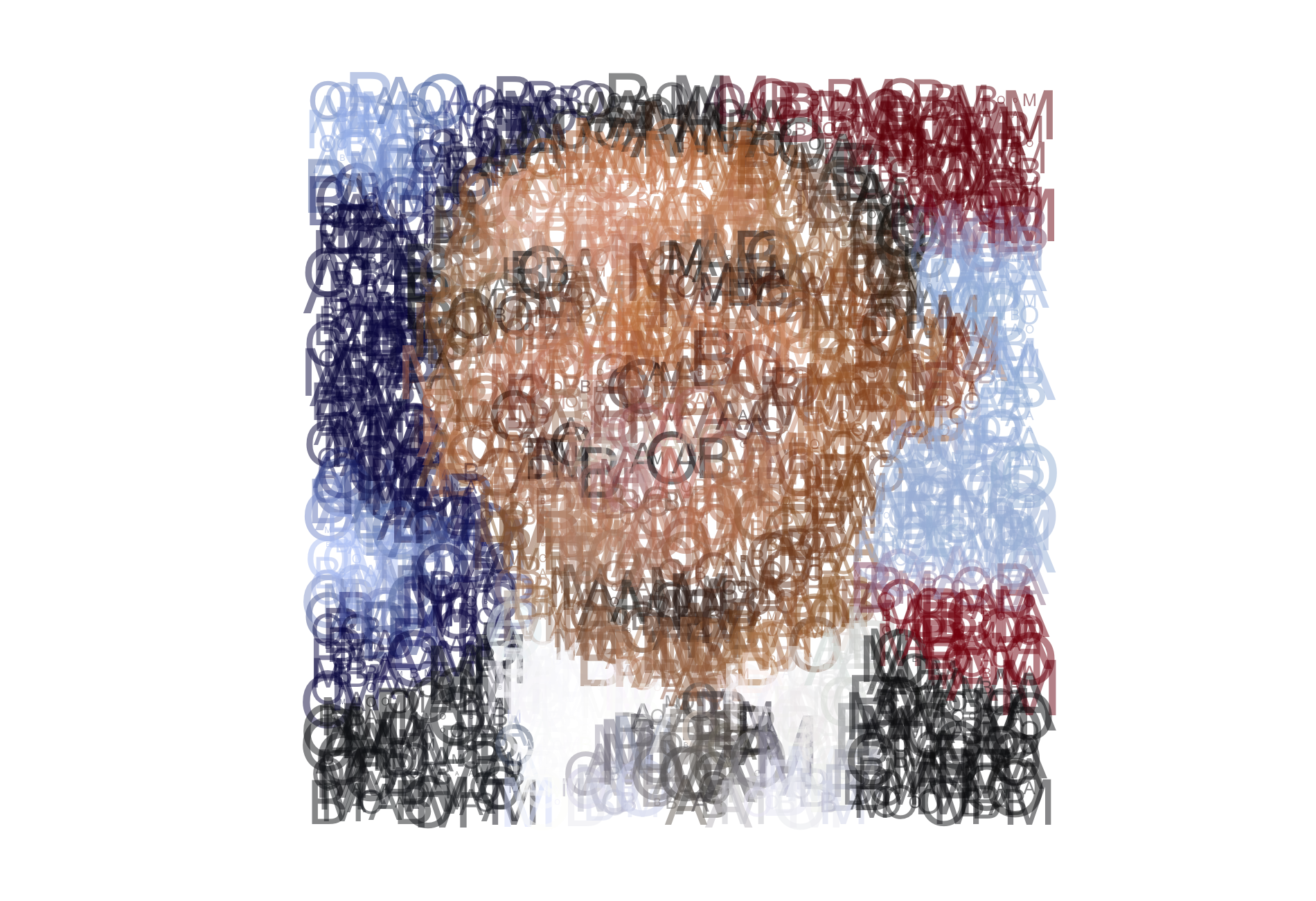
Obama made out of letters
Per the request of @M_T_Patterson and @statsByLopez
The code to generate the following image is below. Enjoy.
library(EBImage)
set.seed(1234)
#im<-readImage("/Users/gregorymatthews/Dropbox/Rart/queenOfHearts.jpeg")
#im<-readImage("/Users/gregorymatthews/Desktop/IMG_9074.jpg")
#im <- readImage("/Users/gregorymatthews/Desktop/guyAlley.jpg")
im <- readImage("/Users/gregorymatthews/Desktop/barry.png")
ddd<-dim(im)
gran<-50
xxx<-round(seq(1,ddd[1],length=gran))
yyy<-round(seq(1,ddd[2],length=gran))
small<-im@.Data[xxx,yyy,]
ddd<-dim(small)

png("/Users/gregorymatthews/barryO.png",h=13,w=19,unit="in",res=100)
plot(0,0,frame.plot=F,xlim=c(0,ddd[1]),ylim=c(0,ddd[2]),col="white",asp=1,xaxt='n',yaxt='n',xlab="",ylab="")

for (i in 1:ddd[1]){print(i)
                    for (j in 1:ddd[2]){
                                        points(i,ddd[2]-j,col=rgb(small[i,j,1],small[i,j,2],small[i,j,3],alpha=0.5),pch=sample(c("O","B","A","M"),1),cex=runif(1,0.5,7))
                    }
}

dev.off()
Cheers.
Fully open-source, transparent implementation of Wins Above Replacement: Results from 2013
Over the past year, I’ve been involved in a project with Ben Baumer (buy his book!) and Shane Jensen in developing an open source, completely transparent version of the (rather opaque) baseball statistic Wins Above Replacement that we’re calling openWAR. We presented our preliminary results this past summer in a talk at JSM and this fall in a poster at NESSIS, but now our full paper is available on ArXiV. (Below you can see the chalkboard that resulted from our initial discussion….I assume this will be historic someday.)

As part of our open source proposal, we’ve also developed an R package, also called openWAR, that allows the user to scrape play by play data from the web and then, if they choose, compute our version of openWAR. The package is currently available on Ben’s github and should be available on CRAN soon. (Jim Albert (!) mentioned this package in his recent book , which you should probably buy even if it didn’t have my name in it. You should buy it twice, since my name is in it.)
Quick story about Jim Albert: When I was deciding where to go to grad school I applied to Bowling Green specifically because Jim Albert was there. I got in and even had an email address and was all set to go, but they couldn’t give me an answer about funding. UConn came along and offered me full funding, and the rest is history. So it’s a pretty big honor for me to be mentioned in Jim Albert’s book.
So what are our results? Below you’ll find out top 20 players for 2013. One interesting thing to note is that according to our openWAR, Trout actually had a better year in 2013 than in 2012 and he still didn’t win the MVP award.
 Here is a comparison of our top 10 players from 2013 versus Fangraph’s top 10 players. Both methods agree that Mike Trout was the best player in 2013, and both methods had Josh Donaldson, Miguel Cabrera, Chris Davis, and Paul Goldschmidt in the top 10.

Next is a table of the ten best and worst fielders of 2013. What you should notice about this is that Miguel Cabrera, according to openWAR, was the worst fielder in baseball in 2013. It’s really incredible that his offensive numbers are so good that they more than compensate for his poor fielding.

The best base runner of 2013 was Ian Kinsler with a RAA of 10.64 and the worst base runner was Victor Martinez. The ninth worst base runner in 2013 was….Miguel Cabrera. Again, think about how good Cabrera has to be as a hitter to overcome his weaknesses as a fielder AND a baserunner to have won TWO AL MVP awards in a row. 
Cheers.
MLB Payroll vs Winning percentage
Dave Cameron over at FanGraphs wrote an interesting article about 2012 payroll and wins. In it, he used a scatterplot, which I assume was made with excel. I’d like to try to persuade everyone to stop making graphics in excel. I’m probably a little bit biased, but R with the ggplot2 package is much, much better. (And it’s easy!) I present to you below, my entire argument for why R with ggplot2 is better than excel:
Here is the code for making this graph
Cheers.
Presidential Candidates, Search Engine Auto-Complete, and Word Clouds: Bicycles, Unicorns, and American Presidential Politics
Finally, I’ve managed to post something that’s not about @BillBarnwell‘s flawed “study” titled “Mere Mortals” (Here’s why he’s wrong. Here is what happens when I apply his logic to something else….you get non-sense). Anyway, here is an update to the presidential candidates search engine auto-complete word clouds (The original post and description of how the data is collected and processed is here).
According to search engines Obama is a gay, socialist/communist, muslim terrorist version of the Antichrist (or possible, not even living thing, but a bicycle), and Romney is an idiot, douche bag, ass hole, mormon unicorn that lies.


Cheers.
Idiots, Liars, and Unicorns: Presidential Politics and Search Engines
In the past I’ve posted search engine auto-completes for some of the presidential candidates. For instance, here are Romney and Obama’s results from 5/30/2012, here are Romney and Obama’s results from 4/16/2012, and here are the republican primary candidates from 12/29/2011. Below you will find the auto-completes for the two presidential candidates from 8/16/2012. I’m also including word clouds now.
I’m using three search engines (Google, Bing, and Yahoo!) and two search terms for each candidate (Mitt Romney, Mitt Romney is, Barack Obama, Barack Obama is). I’m then weighting the terms from 10 to 1 for Google and Yahoo and 8 to 1 for Bing (as they only return 8 search terms), based on the order they appear in the auto-completes. For the first two word clouds, I’m additionally weighting the search engines with Google getting weight 11.7, Bing gets 2.7, and Yahoo gets 2.4. (These numbers are approximately the number, in billions, of searches performed on each site respectively in February 2012.)
The first word cloud represents all of the words with weighting for both presidential candidates. Kind of makes you think a little bit about the political discourse in this country when some of the tops words for presidential candidates are idiot, liar, and antichrist. (For those of you new to the internet, here is the explanation for “your new bicycle”.)

This next word cloud is the same as the previous one, except it is separated by candidate. The blue and red words are Obama and Romney, respectively. If you’re wondering about the “Unicorn” on the Romney side of the word cloud, you may be interested in this facebook page. According to them, “There has never been a conclusive DNA test proving that Mitt Romney is not a unicorn. We have never seen him without his hair — hair that could be covering up a horn. No, we cannot prove it. But we cannot prove that it is not the case.” Truer words have never been spoken….

The final wordcloud of the trio breaks down the auto-complete terms by search engine. Note that, these words for this wordcloud are not weighted by search engine, but they are weighted by order within each search engine. I think it’s kind of interesting that, for Yahoo, the big words are religions: Muslim and Mormon. This makes me wonder if different search engines might predict in some way political affiliation, and, apparently, I’m not the only one who’s thought about this. Looks like a group called Engage has already looked into this and their results are summarized nicely in this graphic. According to them, Googlers tend to be more Democratic and Bingers (?) tend to be more Republican. (I don’t see Yahoo on their graphic, which I find odd.) Also, according to Alexa.com Bing users tend to be older than the average internet user, slightly more likely to have “some college” education, and slightly less likely to have a graduate degree. Google and Yahoo users tend to be very much the average internet user with the exception that they are much less likely to be over the age of 65.

Below here, you’ll find screen shots of the Google, Yahoo, and Bing auto-completes if you’re interested in the raw data that I used.


YAHOO!


BING


Cheers.
Low hit, no hit, and perfect games: The King Felix Edition
Felix Hernandez of the Seattle Mariners just threw the third perfect game of the season, so I figured it was a good time to update my low hit games graphs that I posted in June. So, here they are:

 Cheers.
MLB Rankings – 8/14/2012
StatsInTheWild MLB rankings as of August 6, 2012 at 8:17pm. SOS=strength of schedule
| Team | Rank | Change | Record | ESPN | TeamRankings.com | SOS | Run Diff |
| NYY | 1 | – | 63-44 | 3 | 1 | 5 | +92 |
| Texas | 2 | – | 63-44 | 4 | 2 | 13 | +83 |
| LA Angels | 3 | – | 58-51 | 9 | 6 | 7 | +49 |
| Washington | 4 | ↑2 | 65-43 | 2 | 4 | 23 | +82 |
| ChiSox | 5 | ↑4 | 59-48 | 7 | 5 | 14 | +64 |
| Cincinnati | 6 | ↑5 | 66-42 | 1 | 3 | 29 | +72 |
| Oakland | 7 | ↑1 | 58-50 | 8 | 7 | 8 | +28 |
| Detroit | 8 | ↓1 | 58-50 | 13 | 9 | 12 | +24 |
| TampaBay | 9 | ↑1 | 56-52 | 14 | 12 | 3 | +19 |
| Atlanta | 10 | ↑5 | 62-46 | 5 | 8 | 21 | +62 |
| Boston | 11 | ↓6 | 54-55 | 17 | 13 | 6 | +29 |
| Toronto | 12 | ↓8 | 53-55 | 18 | 14 | 2 | +9 |
| St. Louis | 13 | ↑1 | 59-49 | 10 | 15 | 30 | +110 |
| Baltimore | 14 | ↓2 | 57-51 | 16 | 11 | 1 | -57 |
| Pittsburgh | 15 | ↓2 |
61-46 | 6 | 10 | 28 | +36 |
| Seattle | 16 | ↑1 | 51-59 | 20 | 17 | 4 | -3 |
| Arizona | 17 | ↑4 | 55-53 | 15 | 19 | 26 | +42 |
| SF | 18 | ↓2 | 59-49 | 11 | 16 | 27 | +19 |
| LA Dodgers | 19 | ↓1 |
59-50 | 12 | 18 | 25 | +15 |
| NY Mets | 20 | – | 53-56 | 19 | 20 | 17 | -5 |
| Minnesota | 21 | ↑3 | 47-61 | 25 | 22 | 11 | -79 |
| Kansas City | 22 | – | 45-62 | 26 | 23 | 10 | -60 |
| Cleveland | 23 | ↓4 | 50-58 | 21 | 21 | 9 | -90 |
| Milwaukee | 24 | ↓1 | 48-59 | 22 | 26 | 19 | -13 |
| Philadelphia | 25 | – | 49-59 | 24 | 24 | 19 | -29 |
| Miami | 26 | – | 49-60 | 23 | 25 | 15 | -100 |
| Chic Cubs | 27 | ↑1 | 43-63 | 28 | 27 | 18 | -79 |
| San Diego | 28 | ↓1 | 46-64 | 27 | 28 | 22 | -61 |
| Colorado | 29 | – | 38-68 | 29 | 29 | 20 | -117 |
| Houston | 30 | – | 36-73 | 30 | 30 | 16 | -142 |
Past Rankings:
Cheers.
2012 Olympics – Final Medal Count
Canada is incredible. They somehow managed to win 18 total medal and only 1 gold. Amazing. How is it possible to be so consistently nearly the best? Has anyone ever won more medals with fewer golds?
 Cheers.
